-
Die Evolution der Schärfe: Eine historische Zeitreise mit Capsaicin 🌶️
Das Phänomen der Schärfe beim Essen wird im Alltag meist rein kulinarisch bewertet. Aus evolutionsbiologischer und historischer Sicht handelt es sich dabei jedoch um ein hocheffizientes Abwehrsystem der Natur, das vom Menschen gezielt umgangen und für eigene Zwecke modifiziert wurde.
Die visuelle Telemetrie zeigt die schrittweise Transformation von der unstrukturierten biologischen Rohmasse bis zum finalen Aggregatzustand auf dem Teller.
Das initiale System-Setup vor dem Start
1/60s f/5 ISO 250/25° 16-50mm f/2,8 VR f=30mm/45mm
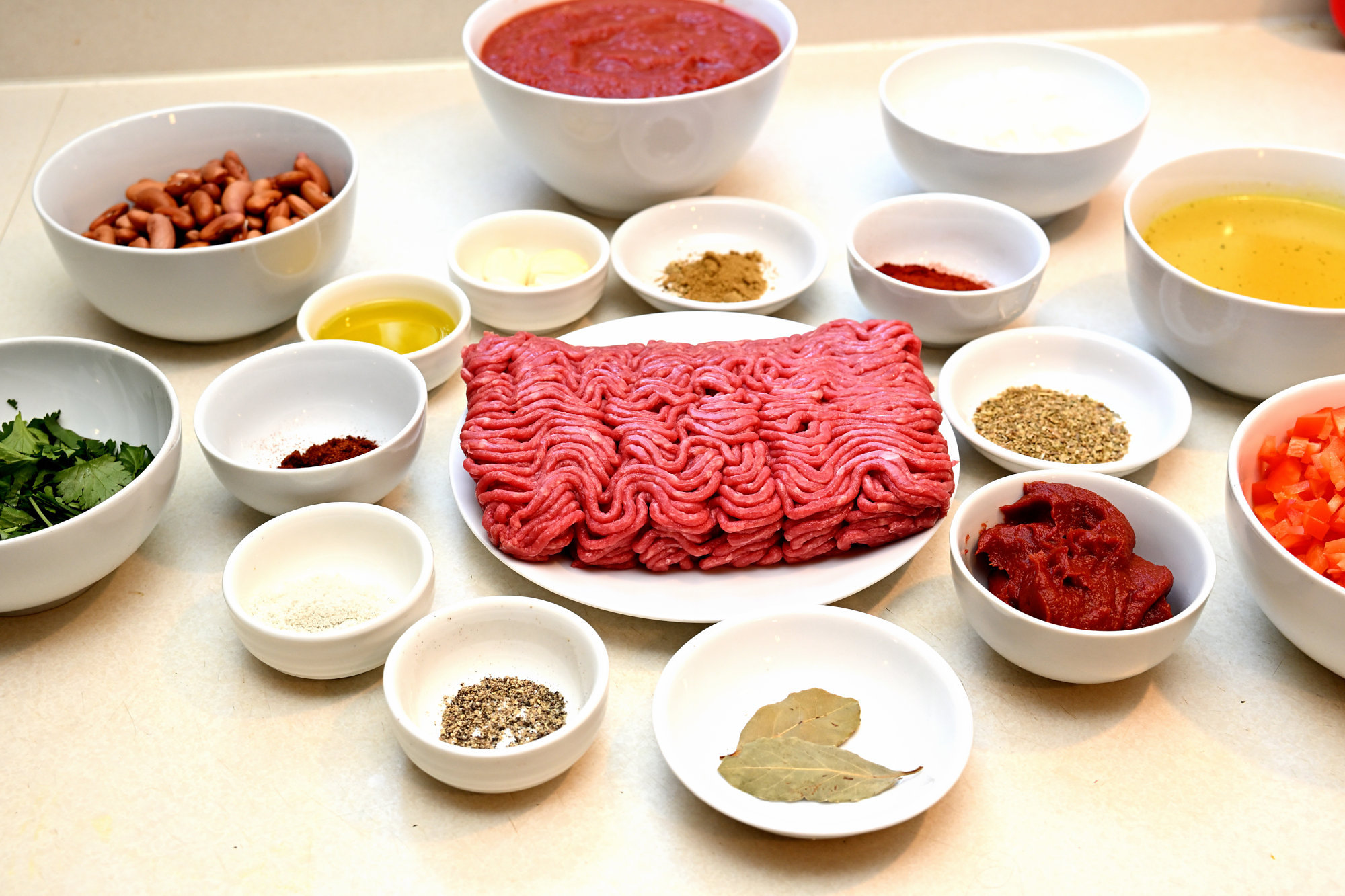
Chilis verdanken ihre Schärfe dem Alkaloid Capsaicin. Aus Sicht der Evolution ist dieser Stoff eine reine Abwehrwaffe. Pflanzen der Gattung Capsicum entwickelten den Mechanismus, um Säugetiere vom Verzehr abzuhalten, da deren Verdauungstrakt die Samen zerstört. Vögel hingegen besitzen keine Rezeptoren für Capsaicin; sie fressen die Früchte unbeschadet und sichern die Evolution der Pflanze durch die unversehrte Ausscheidung der Samen.Thermische Transformation im Kochgefäß
1/60s f/5 ISO 250/25° 16-50mm f/2,8 VR f=22mm/33mm

Die menschliche Reaktion auf diesen Abwehrmechanismus ist paradox: Statt die Pflanze zu meiden, kultiviert die Menschheit Chilis seit fast 10.000 Jahren und züchtet sie systematisch auf höhere Capsaicin-Konzentrationen. Beim Verzehr dockt das Molekül an die TRPV1-Rezeptoren1 der Nervenenden an. Diese sind eigentlich für die Erkennung von thermischer Hitze (ab 43 °C) zuständig. Dem Gehirn wird somit eine akute Verbrennung signalisiert, obwohl keine reale Gewebeschädigung stattfindet.Der biochemische Puffer (die vegetarische Begleitkomponente)
Ein reines Chili stößt schnell an die Grenzen der menschlichen Sensorik. Als funktionale System-Erweiterung auf dem Teller dienen hier selbstgemachte, fleischlose Gemüse-Patties.
1/60s f/5 ISO 250/25° 16-50mm f/2,8 VR f=22mm/33mm

Das ist keine reine Geschmacksentscheidung, sondern angewandte Biochemie: Capsaicin ist extrem lipophil (fettlöslich). Die pflanzlichen Öle und Fette, die beim Anbraten der Patties zum Einsatz kommen, binden das Capsaicin im Mundraum und lösen es sanft von den TRPV1-Rezeptoren. Zusätzlich sorgt diese Kombination für ein biologisches Nährstoff-Upgrade: Die in den Chilis reichlich vorhandenen Vitamine A und E sind ebenfalls fettlöslich. Ohne die Fett-Matrix der angebratenen Gemüse-Patties könnte der menschliche Verdauungstrakt diese essenziellen Verbindungen gar nicht aufspalten und verwerten.Historischer Exkurs: Spuren der globalen Verbreitung
Abseits der Biologie hat die Verbreitung der Schärfe die Weltgeschichte durch höchst eigenwillige Dynamiken beeinflusst:
🌋 Die taktische Barriere der Maya
Bei kriegerischen Auseinandersetzungen verbrannten die Maya getrocknete Chilis im Wind. Der entstehende Rauch wirkte auf die feindlichen Linien wie ein primitives Tränengas. Es gilt als einer der frühesten dokumentierten Einsätze biologischer Reizstoffe in der Kriegsführung.
🦜 Der selektive Gartenfilter
Da die Schärfewahrnehmung bei Vögeln nicht existiert, nutzt die moderne Biologie Capsaicin-Pulver im Vogelfutter. Es fungiert als rein mechanischer Filter: Eichhörnchen und Nagetiere meiden das Futter aufgrund des brennenden Reizes, während Vögel die Nahrung ungestört aufnehmen können.
🧭 Das Pfeffer-Dilemma von Kolumbus
Als Christoph Kolumbus 1492 auf der Suche nach schwarzem Pfeffer in Amerika landete, stieß er auf die scharfen Schoten. Um seine europäischen Geldgeber zu beruhigen und den wirtschaftlichen Erfolg der Expedition zu sichern, deklarierte er sie fälschlicherweise als Verwandte des Pfeffers. Daher stammt die bis heute anhaltende begriffliche Verwirrung im englischen Raum (Chili Pepper).
Die kulinarische Komposition
Am Ende steht ein vollendeter Teller auf dem Tisch. Das Zusammenspiel aus thermischer Hitze und der chemischen Täuschung unseres Nervensystems schließt den Kreis einer jahrtausendealten Evolutionsgeschichte.
Und während das Gehirn noch die simulierte Kernschmelze verarbeitet, meldet der restliche Organismus bereits die mit Abstand beste Mahlzeit der Woche.
1/60s f/5 ISO 250/25° 16-50mm f/2,8 VR f=22mm/33mm


[SYSTEM-LOG: Global release deployment successfully verified at: [0x7B774C:0x1E]]
-
Für die Entdeckung des TRPV1-Capsaicin-Rezeptors wurde 2021 der Nobelpreis für Medizin verliehen. Siehe offizielle Pressemitteilung des Nobelpreiskomitees: The Nobel Prize in Physiology or Medicine 2021. ↩
-
-
Resolving Window Border Glitches During MFC DPI Changes
When developing Windows Desktop applications with C++ and the MFC Ribbon framework (
CMFCRibbonBar), dynamic high-DPI scaling can introduce layout anomalies. A specific issue occurs when moving an application window from a high-DPI display (e.g., 200%) to a lower-DPI display (e.g., 150% or 100%): a transparent or unpainted border appears around the window frames.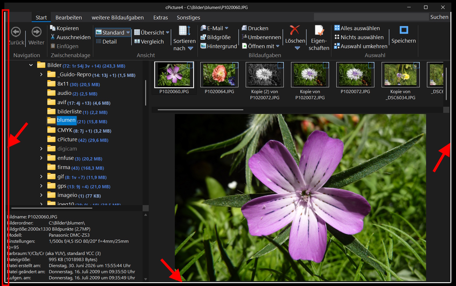
Observed Behavior:
- Initial Start: If the application is launched directly on the lower-DPI monitor, the window dimensions and layout are computed correctly.
- Dynamic Downgrade: The layout anomaly occurs only during a live DPI reduction at runtime.
- Standard Methods: Attempting to force layout updates (
RecalcLayout,UpdateWindow, or invoking custom scaling adjustments) inside theWM_DPI_CHANGEDhandler does not resolve the issue.
Root Cause Analysis
During a dynamic DPI change, the operating system resizes the top-level window. The MFC Ribbon framework modifies the standard window layout by hooking into the Non-Client Area (NC) calculation to implement custom title bars and visual themes.
When downgrading the DPI, a timing mismatch occurs. Windows scales down the outer window bounds, but MFC’s internal metric caches temporarily retain the larger frame dimensions from the previous DPI tier. When Windows sends the
WM_NCCALCSIZEmessage to determine the size of the client area, MFC applies outdated padding values, shifting the client area boundaries inward. Because the outer window has already shrunk, this geometric discrepancy results in an unpainted, transparent margin.Since this calculations happen inside
CFrameWndEx::OnNcCalcSize, adjustments within the standardOnDpiChangedfunction are ineffective. The layout metrics must be corrected where the window boundaries are calculated.
Technical Solution: Intercepting
WM_NCCALCSIZEThe most reliable approach is to utilize the native Windows default window procedure (
DefWindowProc) as a reference point. By passing the message to the OS first, we obtain the mathematically correct border padding for the current DPI tier. We then overwrite the incorrect side-boundary metrics calculated by MFC.By leaving the top boundary (
lpncsp->rgrc.top) unaltered, the MFC Ribbon retains full control over the custom title bar height, while the left, right, and bottom edges are aligned with the native Windows framework.Step 1: Add the handler to your header (
MainFrm.h)// In your CMainFrame class definition afx_msg void OnNcCalcSize(BOOL bCalcValidRects, NCCALCSIZE_PARAMS FAR* lpncsp);Step 2: Register the message in your implementation (
MainFrm.cpp)BEGIN_MESSAGE_MAP(CMainFrame, CFrameWndEx) // ... your other message maps ON_WM_NCCALCSIZE() END_MESSAGE_MAP()Step 3: Implementation
void CMainFrame::OnNcCalcSize(BOOL bCalcValidRects, NCCALCSIZE_PARAMS FAR* lpncsp)
{
    if (bCalcValidRects && lpncsp != NULL)
    {
        // 1. Backup the original outer window dimensions
        RECT rcDefaultWindow = lpncsp->rgrc;

        // 2. Query the native Windows API for correct DPI-scaled boundaries
        ::DefWindowProc(m_hWnd, WM_NCCALCSIZE, bCalcValidRects, reinterpret_cast<LPARAM>(lpncsp));
        RECT rcCorrectClient = lpncsp->rgrc;

        // 3. Restore the original state before invoking MFC
        lpncsp->rgrc = rcDefaultWindow;

        // 4. Invoke the MFC base class for standard Ribbon setup
        CFrameWndEx::OnNcCalcSize(bCalcValidRects, lpncsp);

        // 5. Override the incorrect left, right, and bottom padding metrics.
        // The top value remains managed by MFC for proper title bar height.
        lpncsp->rgrc.left   = rcCorrectClient.left;
        lpncsp->rgrc.right  = rcCorrectClient.right;
        lpncsp->rgrc.bottom = rcCorrectClient.bottom;

        return;
    }

    // Fallback path for invalid parameters
    CFrameWndEx::OnNcCalcSize(bCalcValidRects, lpncsp);
}
Startup and Runtime Performance Impact
Integrating
DefWindowProccalls into the window message structure raises potential concerns regarding application initialization speed and performance optimization.However, this implementation introduces no measurable overhead:
- Algorithmic Execution: Processing
WM_NCCALCSIZEviaDefWindowProcinvolves pure bounding-box arithmetic in memory. It does not trigger disk I/O, graphics rendering pipelines, or CPU context switches. - Low Frequency: The message only fires during structural window changes (creation, maximizing, or dynamic DPI mutations). It does not execute during continuous operations or inside the hot rendering loop (
WM_PAINT), leaving the active runtime performance intact.
By enforcing the operating system metrics for the window boundaries, the outdated MFC caching behavior is bypassed, ensuring correct window dimensions across varying display scaling factors.
-
Der digitale Zombiemodus: Über die organisierte Verkümmerung unserer Neugier 🧠📱
Dopamin auf Knopfdruck
Wir leben in einer Welt, die geistig schleichend verkümmert, und wer heute noch einen Funken echte Kreativität in sich trägt, kann dabei fast schon schmerzhaft zusehen. Jeden Tag blicken wir in Gesichter, die stundenlang vom fahlen Licht ihrer Smartphones erleuchtet werden. Menschen, die im Sekundentakt durch endlose Timelines rutschen, tausende sinnlose Beiträge abklicken, scrollen und wischen.
Das Gehirn wird im Dauerfeuer mit billigen Dopamin-Häppchen gefüttert. Am Ende des Tages bleibt von diesem gigantischen Konsum absolut nichts hängen. Es ist eine organisierte Aufmerksamkeitsökonomie, die uns systematisch die Fähigkeit raubt, uns tief auf eine Sache einzulassen. Die Opfer sind längst so abgestumpft, dass sie den eigenen Verfall gar nicht mehr bemerken. Die Neugier stirbt im Rauschen des Algorithmus.
Vom Konsumenten zum Entdecker

Dabei könnte es so anders sein. Vor kurzem habe ich mitten in der Nacht drei einfache Freihand-Fotos von der partiellen Mondfinsternis gemacht. Ein paar schnelle Schnappschüsse, aus denen man einen standardmäßigen, faden während-ihr-scrollt-Post hätte machen können: "Guck mal, der Mond war dunkel. Like hier." Kurz hochgeladen, kurz abgehakt.
Aber mit dem schnellen Klick muss die Sache ja nicht vorbei sein, wenn man anfängt, sich für die Hintergründe zu interessieren.Vom kollektiven Erblindungsprozess
Statt gemeinsam staunend Neues zu entdecken, starrt man allzu oft isoliert in den eigenen Feed. Die digitale Wüste flutet uns mit belanglosem Müll und lässt uns verlernen, die reale Welt gemeinsam zu betrachten.

Doch wer die Welt mit der Kamera einfängt, sucht meistens nach mehr als nur nach dem nächsten flüchtigen Klick. Statt das Erlebnis einfach nur passiv abzuhaken, lohnt es sich, tiefer zu graben. Aus den paar Bildern kann ganz schnell eine faszinierende Reise durch die Physik unseres Planeten, die Astronomie und die Evolutionsbiologie werden. Es ist absolut faszinierend zu lernen, dass das rote Leuchten des Blutmonds die Summe aller weltweiten Sonnenuntergänge ist. Oder dass Mistkäfer die Milchstraße als Navigations-Turbo nutzen, um ihr leckeres Mittagessen auf dem kürzesten Weg in Sicherheit zu bringen.
Genau hier liegt die Grenze zwischen digitaler Verdummung und echtem Fortschritt. Man sollte moderne Technologie und künstliche Intelligenz genau so nutzen: als unermüdlichen Sparringspartner, der einem hilft, die Welt besser zu verstehen, Fakten zu hinterfragen und die eigene Kreativität anzukurbeln anstatt uns mit dem nächsten Algorithmus-Häppchen zu betäuben.Erwischen verboten
Was in dieser digitalen Wüste am meisten fehlt, ist das gemeinsame Entdecken von Neuem. Früher hat man sich über skurrile Fakten oder faszinierende Phänomene unterhalten und sich gegenseitig inspiriert.

Heute verliert sich dieser Austausch jedoch im Rückzug auf den eigenen, maßgeschneiderten Feed, wodurch das gemeinsame Staunen gegen virtuelle Berieselung eingetauscht wird.Das Methusalem-Paradoxon

Besonders skurril wird es, wenn man die ältere Generation beobachtet. Man sollte meinen, wer die sechzig überschritten hat, nutzt seine hart erarbeitete Lebensweisheit als Schutzschild gegen diesen digitalen Unfug. Doch Pustekuchen. Statt altersweiser Gelassenheit sieht man oft dieselbe Abstumpfung wie bei der TikTok-Jugend. Da stellt sich unweigerlich die kritische Frage: Was haben diese Leute eigentlich im Leben gelernt? Wo ist die Weisheit geblieben, wenn man am Ende doch nur wieder genauso blöd vor dem Bildschirm sitzt wie früher?Wir ertappen uns ja alle hin und wieder selbst dabei, wie wir kostbare Lebenszeit an sinnlose Klicks verschwenden. Man muss über diese eigene Schwäche auch einfach mal lachen können. Aber genau das ist der Punkt: Wer über sich selbst lachen kann, hat zumindest noch ein Fünkchen Bewusstsein übrig. Der Rest scrollt einfach stumm weiter ins geistige Nirwana.
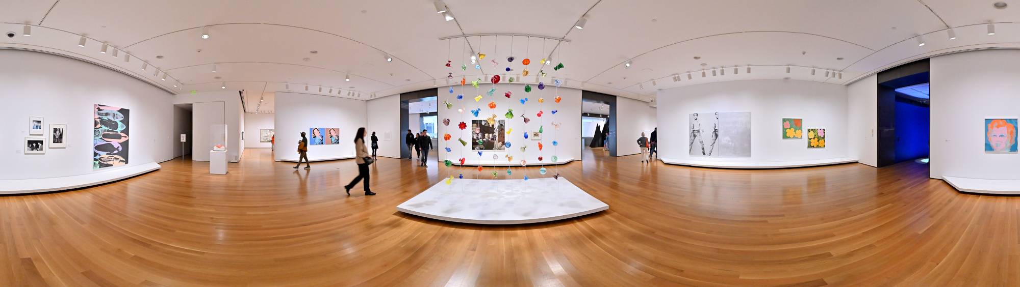
Wir müssen lernen, Technologie wieder als Werkzeug für unsere echte, kindliche Neugier zu begreifen. Wenn du das nächste Mal etwas siehst, das dein Interesse weckt, sei es der Mond am Himmel, ein seltsames Insekt auf dem Boden oder eine verrückte Struktur in der Natur: Klick nicht weiter. Nutz die Werkzeuge, die dir zur Verfügung stehen, um zu lernen, zu hinterfragen und zu kreieren.

Der geistige Verfall um uns herum passiert nur dann, wenn wir aufhören, selbst zu denken. Bleibt kreativ unruhig. Es gibt da draußen viel zu viel zu entdecken, um es für ein paar parataktische Häppchen auf dem Bildschirm einzutauschen. -
Mondfinsternis
Heute Nacht gab es oben am Himmel ein spannendes Alternativprogramm zum strahlenden Vollmond.
Traditionell wird der August-Vollmond auch als Störmond bezeichnet, und wenn sich die Erde genau zwischen Sonne und Mond schiebt und ihren Schatten wirft, sieht das Ganze gleich viel spannender aus. Wegen der partiellen Mondfinsternis hatte mir da mehr einen Sparmond mit dem charakteristischen hellen Rand. Weltweit passiert das zwar zwei- bis dreimal im Jahr, aber man muss ja trotzdem im richtigen Moment auch hinschauen.Ich habe mir kurzentschlossen die Nikon Z50II mit dem 50-250mm Objektiv geschnappt. Eigentlich gehört sich für Astrofotografie ja ein fettes Stativ. Dank gutem Bildstabilisator und ordentlich Luftanhalten ging das Ganze diesmal aber auch erstaunlich gut freihändig durch. Nach kurzer Zeit war der Moment dann auch schon wieder vorbei.
Der Erstkontakt:
1/25s f/6,32 ISO 6400/39° 50-250mm f/4,5-6,3 VR f=250mm/375mm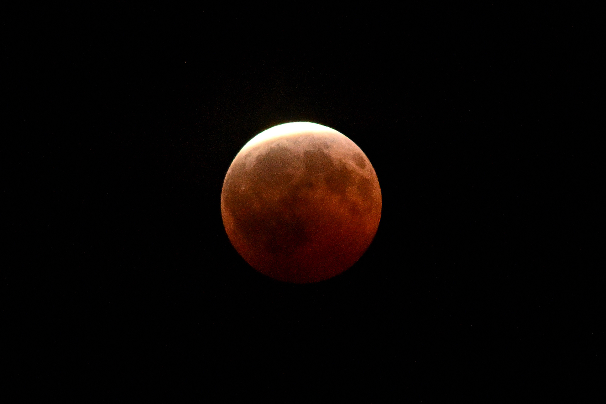
3 Minuten später:
1/25s f/6,3 ISO 2500/35° 50-250mm f/4,5-6,3 VR f=250mm/375mm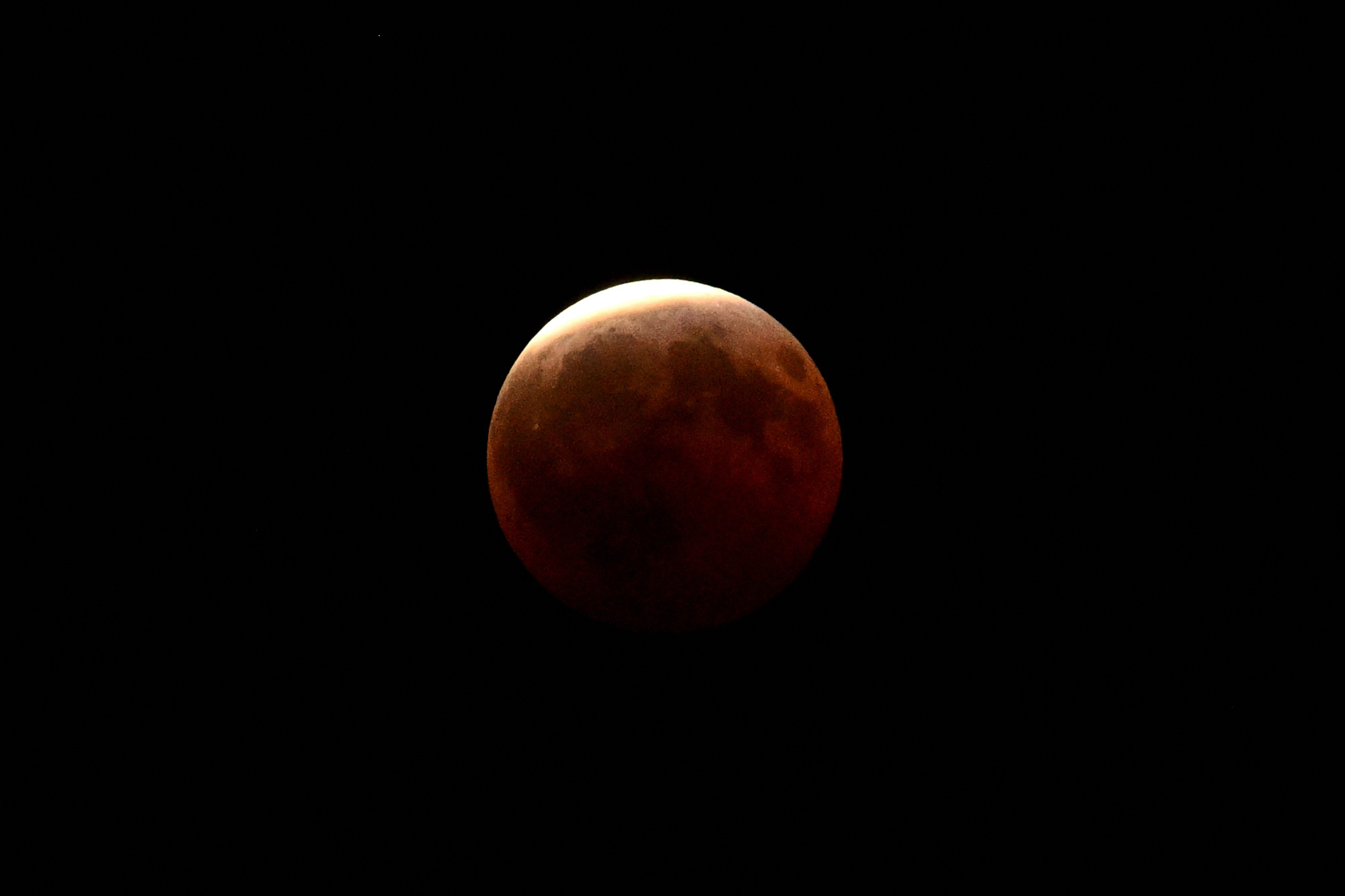
nochmal 3 Minuten später, immer noch da:
1/15s f/6,3 ISO 1250/32° 50-250mm f/4,5-6,3 VR f=250mm/375mm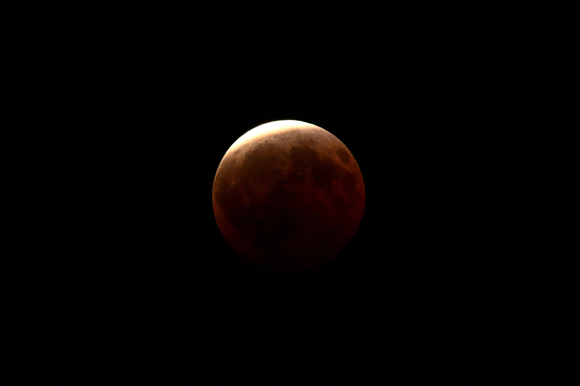
Viel länger hätte ich die Luft eh nicht anhalten können. Kurz darauf haben die Nachbarbäume die Sichtachse zensiert, weil sie wohl unbedingt auch mit aufs Bild wollten.
Aber die Finsternis ist nicht nur für Sternengucker spannend, sie verändert die ganze Natur:
🪲
Mistkäfer nutzen als weltweit einzige bekannte Lebewesen das schwache Lichtband der Milchstraße, um dank hochempfindlicher Facettenaugen nachts perfekt geradeaus zu navigieren. Weil das störende, helle Mondlicht plötzlich weggedimmt wird, sehen sie die Galaxie viel besser, legen den intergalaktischen Vorwärtsgang ein und rollen ihre Dungkugeln3 plötzlich dreimal schneller und präziser als in jeder normalen Vollmondnacht.🌋
Das rote Leuchten des Blutmonds ist die Summe aller Sonnenuntergänge der Erde. Die Atmosphäre wirkt wie ein gigantisches Prisma und projiziert das weltweite Abendrot direkt auf den Mond. Gleichzeitig sackt die Temperatur dort oben so schlagartig ab, dass der Mond schrumpft und messbare Mondbeben ausgelöst werden.⛵
Im Jahr 1504 rettete eine Mondfinsternis Christoph Kolumbus das Leben. Als die Ureinwohner auf Jamaika ihm keine Vorräte mehr geben wollten, drohte er ihnen an, Gott würde dem Mond das Licht stehlen. Als die Finsternis wie vorhergesagt eintraf, gaben die verängstigten Inselbewohner ihm sofort alles, was er brauchte.
-
Hab doch tatsächlich versucht, die Blende auf 2,8 hochzudrehen. Vollmond halt. ↩
-
Das Logistik-Unternehmen Dungtransport ist pure Lebensversicherung: Frischer Dung liefert wichtige Nährstoffe, sorgt am Haufen aber für ordentlich Gedränge. Um den Proviant nicht an die Konkurrenz zu verlieren, formen sie blitzschnell eine Kugel, flüchten auf dem absolut schnellsten Weg (daher die gerade Linie via Milchstraße) und vergraben das leckere Mittagessen als ungestörtes Festmahl oder exklusive Kinderstube für den Nachwuchs.
Mehr Details zu diesem Orientierungsverfahren gibt es im Wikipedia-Eintrag zum Mistkäfer und in der wissenschaftlichen Originalstudie von Marie Dacke auf ScienceDirect. ↩
-
-
Surfen auf der Raumwelle: Wellendynamik, Tageszeiten und Antennenformen der Kurzwelle
Das unsichtbare Uhrwerk der Kurzwelle: Wellendynamik, Tageszeiten und Antennenformen
Wer sich nach den ersten Gehversuchen im Antennenbau tiefer in die Welt der Kurzwelle (3 bis 30 MHz) begibt, stellt schnell fest: Die Kurzwelle schläft nie, aber sie verändert stündlich ihr Gesicht. Während ein UKW-Signal stur und verlässlich bis zum Horizont wandert, gleicht die Kurzwelle einem dynamischen Organismus. Bänder, die mittags vor Signalen fast überlaufen, sind nachts plötzlich wie leergefegt, nur um Platz für weltweite Verbindungen auf Frequenzen zu machen, die tagsüber völlig unbrauchbar schienen.
Um dieses Zusammenspiel aus solarer Strahlung, Frequenz und Zeit ohne langes Suchen zu durchschauen, lässt sich die Dynamik der Ionosphäre in einer zentralen Matrix zusammenfassen.
Die Ausbreitungs-Matrix: Frequenz vs. Tageszeit
Frequenzbereich Tagsüber (Starke Sonne ☀️) Nachts (Keine Sonne 🌙) Physikalisches Phänomen in der Praxis Obere Kurzwelle
(14 - 30 MHz)
• 20m, 15m, 10mPerfekt für DX (Weitverkehr):
Die Wellen durchbrechen die D-Schicht mühelos und werden von der geladenen F-Schicht flach reflektiert.Völlig tot (Offen ins All):
Ohne Sonne verliert die F-Schicht ihre Ladung. Die schnellen Wellen fliegen ungebremst ins Weltall.Reine Tagbänder. Perfekt für interkontinentale Verbindungen, solange die Sonne scheint. Macht nach Sonnenuntergang rasant dicht. Mittlere Kurzwelle
(7 MHz)
• 40mDas NVIS-Arbeitspferd:
Hoch genug, um die D-Schicht zu durchdringen, aber niedrig genug für Steilstrahlung (NVIS) an der F-Schicht.Das DX-Arbeitspferd:
Für Steilstrahlung zu hoch (Signal entweicht), aber bei flachen Winkeln spiegelt die Restladung für weltweiten Funk.Das Chamäleon. Tagsüber die erste Wahl für den regionalen Nahverkehr (0-500 km), nachts öffnet es sich für den weltweiten Funkverkehr. Untere Kurzwelle
(1,8 - 3,5 MHz)
• 160m, 80mKomplett blockiert (Dämpfung):
Die Wellen regen freie Elektronen in der dichten D-Schicht an. Die Energie verpufft komplett als Wärme.Perfekt für NVIS & DX:
Die D-Schicht löst sich nachts auf. Die schwache Nacht-F-Schicht reicht für diese Wellen zur Totalreflexion.Reine Nachtbänder. Tagsüber herrscht hier bis auf die ultrakurze Bodenwelle absolute Stille. Nachts das primäre Band für den Nahbereich.
Faszinierende Anomalien: Wenn die Physik die Regeln beugt
Hinter dieser Matrix steckt die Wechselwirkung aus der solaren UV- und Röntgenstrahlung und den Gasmolekülen unserer Atmosphäre. Doch die Natur hält sich nicht immer an starre Zeitpläne. Drei Phänomene zeigen, wie faszinierend die Dynamik der Raumwelle ist:
1. Das Phänomen der Graulinie (Greyline Propagation)
Zweimal am Tag passiert auf der Erde etwas Magisches: Die Dämmerungszone (der Terminator) wandert als schmaler Streifen um den Globus. In diesem Bereich ist die Sonne am Boden bereits untergegangen (oder geht gerade auf), wodurch sich die blockierende D-Schicht blitzschnell auflöst. Gleichzeitig steht die hunderte Kilometer höhere F2-Schicht noch vollem Sonnenlicht und ist maximal ionisiert.
Für den Funker bedeutet das: Signale auf den niedrigeren Bändern (wie 40m oder 80m) können sich entlang dieser "grauen Linie" mit extrem geringer Dämpfung um die halbe Erde tasten. Es entstehen für wenige Minuten hocheffiziente Funkwege zwischen Regionen, die eigentlich auf der Nachtseite liegen, und solchen, die gerade erwachen.
Exkurs: Warum absorbiert nur die D-Schicht die niedrigen Frequenzen?
Ein Paradoxon des Funks: Die D-Schicht weist die geringste Elektronendichte (Ionisierung) aller Schichten auf, aber warum verursacht ausgerechnet sie am Tag eine so starke Dämpfung der längeren Wellen (wie auf dem 80m- oder 160m-Band), während die viel stärker ionisierten E- und F-Schichten das Signal passieren lassen?
Der Grund liegt in der Dichte der umgebenden Atmosphäre:
- In der D-Schicht (ca. 60-90 km Höhe): Hier ist die Erdatmosphäre noch vergleichsweise dicht. Es befindet sich dort eine hohe Anzahl neutraler Gasmoleküle. Wenn eine niedrige Funkfrequenz eintrifft, bringt sie die freien Elektronen zum Schwingen. Aufgrund der geringen Abstände kollidieren diese schwingenden Elektronen ständig mit den trägen Gasmolekülen. Bei jedem Zusammenstoß wird die Bewegungsenergie der Elektronen in Wärme umgewandelt und die Funkwelle wird dadurch stark gedämpft (Absorption).
- In den höheren E- und F-Schichten (ab 100 km Höhe): In diesen Höhen herrscht ein extremes Vakuum, die Luft ist extrem dünn. Wenn die Funkwelle die Elektronen dort zum Schwingen bringt, bewegen sich diese nahezu ungehindert. Mangels Masse kommt es kaum zu Kollisionen mit Gasmolekülen, wodurch auch keine Energie in Wärme umgewandelt wird. Die Elektronen können die Welle sauber brechen und zur Erde zurückreflektieren (Refraktion).
Zusammenfassend: Niedrige Frequenzen regen die Elektronen zu größeren Schwingungsamplituden an. In der relativ dichten Atmosphäre der D-Schicht führt dies zu einer hohen Kollisionsrate und somit zu hohen Energieverlusten. In den dünneren, höheren Schichten bleibt diese Dämpfung aus, wodurch das Signal ungestört reflektiert werden kann.
2. Die Winteranomalie (Winter Anomaly)
Man sollte intuitiv erwarten, dass die Ionosphäre im Sommer am stärksten ionisiert ist, da die Sonne dann am höchsten steht. Auf den oberen Bändern (wie 20m oder 10m) beobachtet man jedoch das Gegenteil: Die höchsten Grenzfrequenzen tagsüber werden oft im Spätherbst und Winter erreicht.
Der Grund liegt in der Thermodynamik der Atmosphäre und einem Phänomen, das es hier unten bei uns auf der Erde gar nicht gibt: Dem Verhältnis von Molekülen zu freien Atomen:
- Das physikalische Geheimnis: Hier unten am Boden existieren Gase wie Sauerstoff ($O_2$) oder Stickstoff ($N_2$) fast nur als "Paare" (Moleküle). In über 100 km Höhe bricht die starke UV-Strahlung der Sonne diese Paare jedoch auseinander. Es entstehen "Singles", sogenannte freie, ungebundene Atome (einzelner Sauerstoff $O$), die völlig losgelöst durchs All fliegen.
- Im Sommer: Die Sonne heizt die obere Atmosphäre stark auf, wodurch sie sich ausdehnt. Durch diese globale Zirkulation werden die schweren, trägen Gas-Paare (Moleküle) aus tieferen Schichten nach oben in die F-Schicht transportiert. Das Verhältnis von Singles zu Paaren sinkt. Da diese Moleküle freie Elektronen wie ein Schwamm aufsaugen und rekombinieren, sinkt die Elektronendichte, unser Funksignal verliert seinen Spiegel.
- Im Winter: Die obere Atmosphäre kühlt ab und zieht sich zusammen. In der F-Schicht dominieren nun die leichten Singles (freie Sauerstoff-Atome $O$). Da diese einzelnen Atome die Elektronen in Ruhe lassen, bleibt die freie Elektronendichte trotz weniger Sonnenstunden extrem hoch.
Das Ergebnis ist eine hocheffiziente Reflektion hoher Frequenzen mitten im tiefsten Winter.
3. Sporadic-E ($E_s$): Der Sommer-Joker
Gelegentlich bildet sich im Sommer (Mai bis August) in einer Höhe von ca. 90 bis 120 km, also mitten in der eigentlich unbedeutenden E-Schicht, eine wolkenartige, extrem dichte Ionisation aus. Dieses Phänomen nennt sich Sporadic-E.
Die Ursache liegt meist in einer Kombination aus Höhenwinden (Scherwinden) und Meteorenstaub. Diese Wolken sind so dicht, dass sie selbst Frequenzen reflektieren, die sonst nie von der Ionosphäre zurückgeworfen werden: das 10m-Band mutiert zum lokalen Kraftpaket, und selbst VHF-Signale im 6m- oder 2m-Band (inklusive des UKW-Rundfunks) spiegeln sich plötzlich über tausende Kilometer. Das Phänomen taucht unvorhersehbar auf und verschwindet oft nach wenigen Stunden wieder.
4. Die solare Aktivität: Sonnenfleckenzyklus und Ausbreitungsbedingungen
Die Eigenschaften der Ionosphäre hängen maßgeblich vom ca. 11-jährigen Sonnenfleckenzyklus ab. Die Anzahl der Sonnenflecken (Sonnenflecken-Relativzahl) ist ein direkter Indikator für die Intensität der solaren UV- und Röntgenstrahlung, welche die Ionisation der Erdatmosphäre steuert. Veränderungen in dieser Aktivität wirken sich stark auf die Nutzbarkeit der Frequenzbänder aus, führen in der Praxis jedoch auch zu scheinbaren Widersprüchen.
- Die oberen Bänder (15m, 12m und das 10m-Band im Extremfall): Bei einer hohen Anzahl von Sonnenflecken steigt die Elektronendichte in der F-Schicht deutlich an. Dadurch verschiebt sich die maximale nutzbare Frequenz (MUF: Maximum Usable Frequency) nach oben. Das 10-Meter-Band reagiert hierbei am empfindlichsten: Im solaren Maximum mutiert es zum hocheffizienten DX-Band, auf dem weltweite Kontakte mit minimaler Leistung gelingen. In Phasen geringer solaren Aktivität (Sonnenfleckenminimum) kehrt sich dieser Effekt jedoch um. Da die Ionisation der oberen Schichten dann nicht ausreicht, um diese Frequenzen zu reflektieren, sind die Bänder im Bereich von 21 MHz und höher (15, 12 und 10 Meter) die unzuverlässigsten Frequenzbereiche für Weitverbindungen. Das 10m-Band bleibt abseits von Sporadic-E im Sommer oft jahrelang für den DX-Verkehr geschlossen.
- Die unteren Bänder als Profiteure des Minimums (80m- und 160m-Band): Während die oberen Bänder im solaren Minimum an Leistungsfähigkeit verlieren, schlägt die Stunde der unteren Kurzwelle. Im Sonnenfleckenmaximum sorgt die hohe solare Strahlung dafür, dass die tiefe D-Schicht tagsüber extrem stark ionisiert ist und niedrige Frequenzen komplett dämpft. Selbst nachts bleibt oft eine spürbare Restdämpfung und Unruhe im Erdmagnetfeld bestehen. Im Sonnenfleckenminimum hingegen baut sich die blockierende D-Schicht nach Sonnenuntergang extrem schnell und vollständig ab. Gepaart mit einem ruhigen Magnetfeld bietet das solare Minimum daher die historisch besten DX-Bedingungen für das 80-Meter- und insbesondere das 160-Meter-Band, da Signale nachts mit minimalen Verlusten an der F-Schicht reflektiert werden.
- Erhöhte Dämpfung und Radio Blackouts: Unabhängig von den Basisbedingungen bringt eine hohe solare Aktivität spontane Einschränkungen mit sich. Solare Eruptionen (Solar Flares) führen zu einer schlagartigen, extremen Ionisation der dichten D-Schicht. Da diese Schicht aufgrund der höheren Teilchendichte stark absorbierend wirkt (wie im Exkurs oben beschrieben), werden niedrigere Frequenzen komplett gedämpft. Bei starken Ausbrüchen kommt es zum sogenannten Mögel-Dellinger-Effekt (Shortwave Fadeout), bei dem der Funkverkehr auf der Tagseite der Erde zeitweise vollständig zusammenbricht.
Die Kontroverse: Hoher Solar Flux (SFI) ohne verbesserte Bedingungen In der Funkpraxis führt die Interpretation der solaren Messwerte regelmäßig zu Diskussionen. Ein hoher Solar Flux Index (SFI) gilt allgemein als Indikator für hervorragende DX-Bedingungen. Dennoch kommt es vor, dass die Bänder trotz Rekordwerten der Sonne geschlossen bleiben oder die Signale stark gedämpft sind.
Dieser Widerspruch entsteht meist durch das Zusammenspiel mit geomagnetischen Stürmen, die oft auf solare Eruptionen folgen. Diese Stürme stören das Erdmagnetfeld und führen zu einer Depression der F2-Schicht und die Elektronendichte sinkt lokal ab, anstatt zu steigen. Zudem kann die physikalische Aufheizung der oberen Atmosphäre im Sommer (analog zur Winteranomalie) die Rekombination der Elektronen beschleunigen. Ein hoher Fleckenindex ist daher keine isolierte Garantie für offene Bänder, sondern muss immer im Kontext der geomagnetischen Aktivität (K-Index) und der saisonalen Thermodynamik betrachtet werden.
Das Antennen-Szenario: Die Werkzeuge für die Kurzwelle
Während die Endfed-Antenne ein guter Allrounder ist, erfordern spezifische Anwendungen angepasste Geometrien und Antennenformen, die andere Anpassungsnetzwerke als unser 9:1 Unun benötigen.
- Kurz erklärt: Was ist ein Unun? Der Begriff steht für Unbalanced-to-Unbalanced (unsymmetrisch auf unsymmetrisch). Es ist ein Hochfrequenz-Transformator, der die Impedanz (den Widerstand) zwischen einer unsymmetrischen Antenne (wie einer Endfed, die ein Gegengewicht oder die Erde nutzt) und dem unsymmetrischen Koaxialkabel anpasst. Er wandelt nur den Widerstand um, ändert aber nichts an der Symmetrie.
- Der Unterschied zum Balun: Ein Balun hingegen verbindet eine Balanced (symmetrische Antenne wie einen Dipol mit zwei gleichen Schenkeln) mit dem Unbalanced (unsymmetrischen) Koaxialkabel.
Hier sehen wir, wie sich andere klassische Antennenformen im Vergleich zu unserem Endfed-Setup schlagen:
1. Der klassische Halbwellen-Dipol ($\lambda/2$)
Der im Zentrum gespeiste Dipol benötigt keinen 9:1 Unun, da seine Fußpunktimpedanz bereits bei ca. 50-73 $\Omega$ liegt. Er ist ein exzellentes Werkzeug für Richtfunk (DX) bei ausreichender Höhe (mindestens $\lambda/2$). Für den Nahbereich (NVIS) gilt die Faustformel: Die Antenne erzielt die besten Ergebnisse, wenn sie in einer Höhe zwischen $0{,}1\,\lambda$ und $0{,}2\,\lambda$ über dem Boden installiert wird (beim 40m-Band entspricht das genau einer Höhe von ca. 4 bis 8 Metern). Wird sie noch tiefer abgesenkt, steigen die Erdverluste durch die kapazitive Kopplung massiv an und absorbieren einen Großteil der Sendeleistung.
2. Die Magnetische Loop-Antenne (MagLoop)
Diese platzsparende, rauscharme Antenne nutzt einen Drehkondensator zur Abstimmung, was sie ideal für den Balkon macht. Aufgrund ihrer hohen Schmalbandigkeit muss sie bei Frequenzwechseln nachgestimmt werden. Die Einkopplung erfolgt hier meist direkt, ohne den 9:1 Unun.
3. Die Vertikal-Antenne (Groundplane)
Mit einer Länge von $\lambda/4$ und Radials strahlt die Vertikalantenne flach ab und ist ideal für DX auf oberen Bändern. Sie weist eine niedrige Impedanz (30-50 $\Omega$) auf und wird direkt über ein 50 $\Omega$ Koaxialkabel gespeist, nicht über den 9:1 Unun.
4. Die Delta Loop
Diese einwellenlange ($\lambda$) Dreieckantenne vereint geringes Rauschen mit flachem Abstrahlwinkel. Mit einer Impedanz von 100-150 $\Omega$ ist sie für den 9:1 Unun ungeeignet; stattdessen werden 2:1 oder 4:1 Baluns eingesetzt. Sie bietet zudem flexible Polarisationsmöglichkeiten für NVIS oder DX.
Fazit
Wer die Kurzwelle beherrschen will, baut nicht einfach nur eine Antenne, er lernt, das unsichtbare Uhrwerk der Erde zu lesen. Wer weiß, zu welcher Stunde die D-Schicht schläft, wann die F-Schicht das Tor zum Weltall öffnet und welche Antennenform den passenden Winkel in den Himmel meißelt, für den wird die Kurzwelle zu einem faszinierenden, weltumspannenden Spielplatz der Physik.
Seite 1 von 57
Ältere Beiträge →