-
A Cat at Dusk, ISO 12800
Not every improvement in technology needs a big explanation. Sometimes it is just there in a simple picture taken late in the day, when the light is already fading and everything feels a little softer.
These two photos of our cat were taken at dusk with the Nikon Z50 at ISO 12800 and f/2.8. What I like about them is how calm and natural they feel. The images are sharp, the detail is there, and the whole scene keeps its quiet evening mood.
That is one of the nice things about modern cameras. They make this kind of picture easier and leave more room to focus on the subject, the light, and the moment.
Two quiet moments in the fading evening light
1/80s f/2,8 ISO 12800/42° 16-50mm f/2,8 VR f=50mm/75mm

1/80s f/2,8 ISO 12800/42° 16-50mm f/2,8 VR f=50mm/75mm

A closer look at the detail, and a nice reminder of how well this works these days.

From the Z50 to JPEG for the web via Nikon NX Studio, with everything left at the default settings.
-
Zwischen Code und Wok: Chow Mein
Chow Mein aus dem Wok 🍜
Nicht alles muss aus Code, Tools und Builds bestehen. Manchmal ist es ganz gut, zwischendurch etwas zu machen, das genauso viel Struktur hat, aber deutlich besser riecht. Diesmal: Chow Mein, also gebratene asiatische Nudeln mit viel Gemüse, Hitze aus dem Wok und genau diesem kurzen Moment, in dem aus einzelnen Zutaten plötzlich ein richtiges Gericht wird.
Ich mag an solchen Gerichten, dass sie schnell wirken, aber trotzdem präzise sind. Alles wird vorbereitet, liegt bereit, und dann geht es Schlag auf Schlag. Fast ein bisschen wie bei einem Deployment: Wenn das Setup stimmt, läuft der Rest sauber durch. Nur eben mit Knoblauch, Sojasauce und Sesamöl statt Logs und Pipelines.
Am Ende ist Chow Mein genau das, was gute Küche oft ist: unkompliziert, direkt und voller Aroma. Hier ein paar Bilder vom Entstehen.
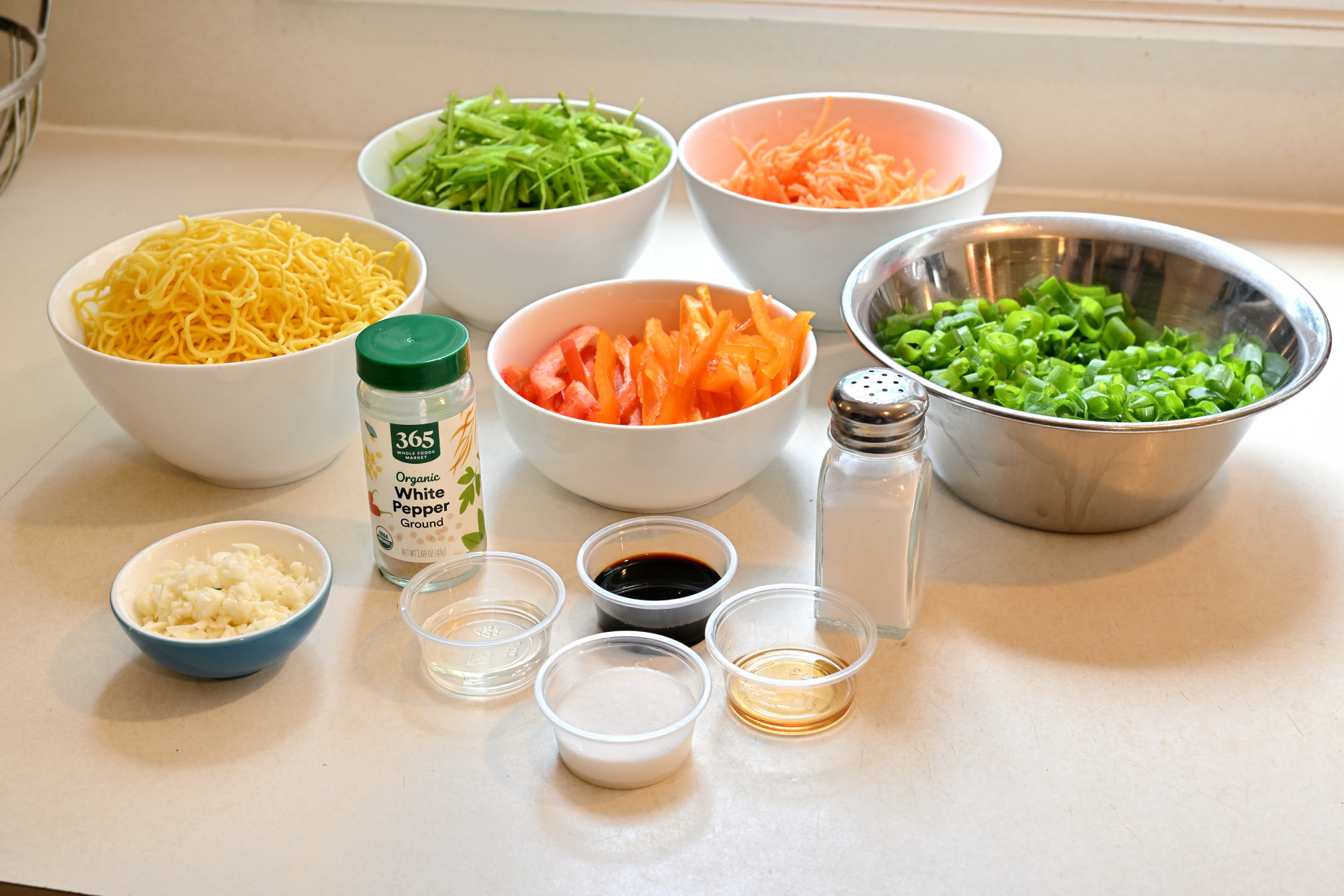
Alle Zutaten im Überblick
Bevor der Wok heiß wird, kommt erst einmal Ordnung auf die Arbeitsfläche: Nudeln, Gemüse, Sauce und alles, was später in wenigen Minuten zusammenfinden soll. Bei so einem Gericht ist die Vorbereitung fast die halbe Miete.
1/40s f/5,6 ISO 100/21° 16-50mm f/2,8 VR f=32mm/48mm
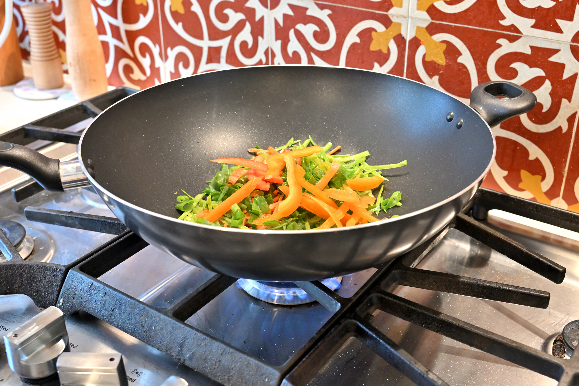
Im Wok: die ersten Schritte
Jetzt wird es ernst. Das Gemüse kommt in den heißen Wok, alles bleibt in Bewegung, und nach den ersten Sekunden entsteht schon dieser typische Duft, bei dem klar ist: Das wird gut.
1/40s f/5 ISO 800/30° 16-50mm f/2,8 VR f=24mm/36mm
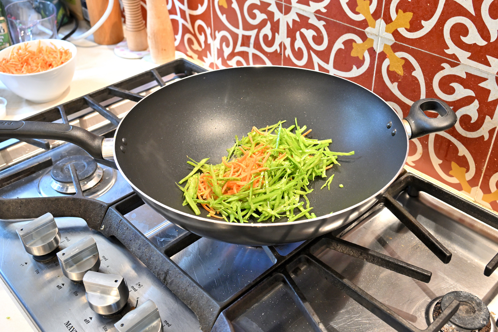
1/40s f/5 ISO 800/30° 16-50mm f/2,8 VR f=28mm/42mm
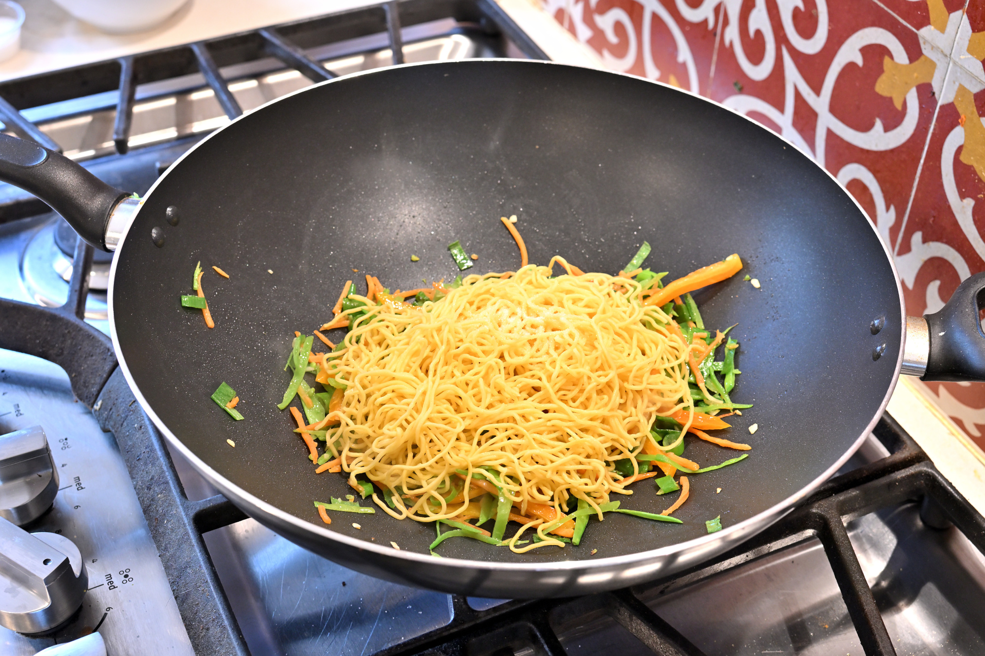
Im Wok: Nudeln und Sauce dazu
Sobald die Nudeln dazukommen, wird aus Vorbereitung ein Gericht. Die Sauce verbindet alles, der Wok gibt Röstaromen dazu, und plötzlich sieht es nicht mehr nach Zutaten aus, sondern nach Abendessen.
1/40s f/5 ISO 500/28° 16-50mm f/2,8 VR f=32mm/48mm
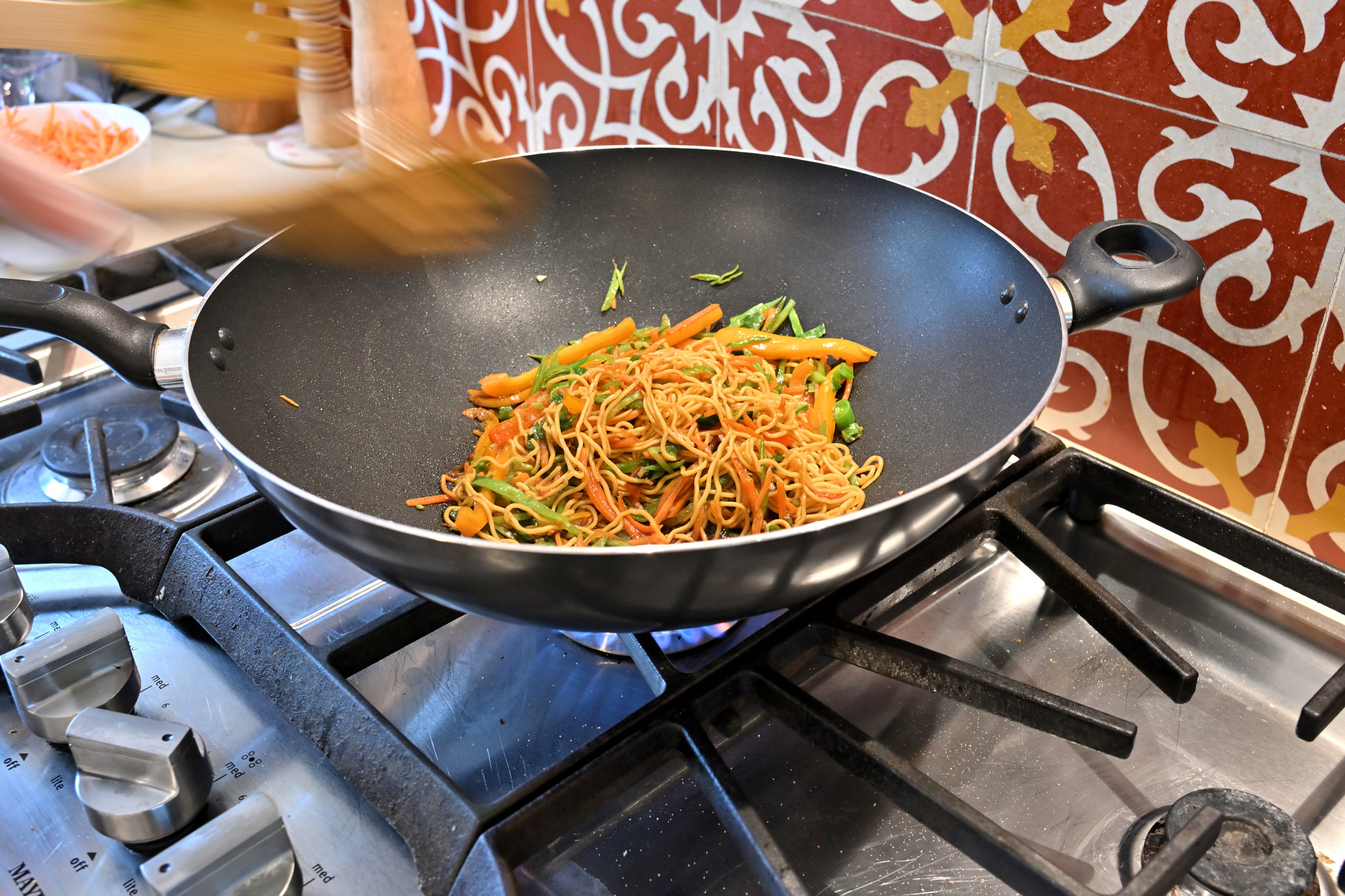
Kurz vor dem Finale
Jetzt passt alles zusammen: Farbe, Struktur und genau die Mischung aus gebraten, saftig und leicht karamellisiert, die Chow Mein ausmacht. Noch ein letzter Schwung im Wok, dann kann angerichtet werden.
1/40s f/5 ISO 500/28° 16-50mm f/2,8 VR f=24mm/36mm
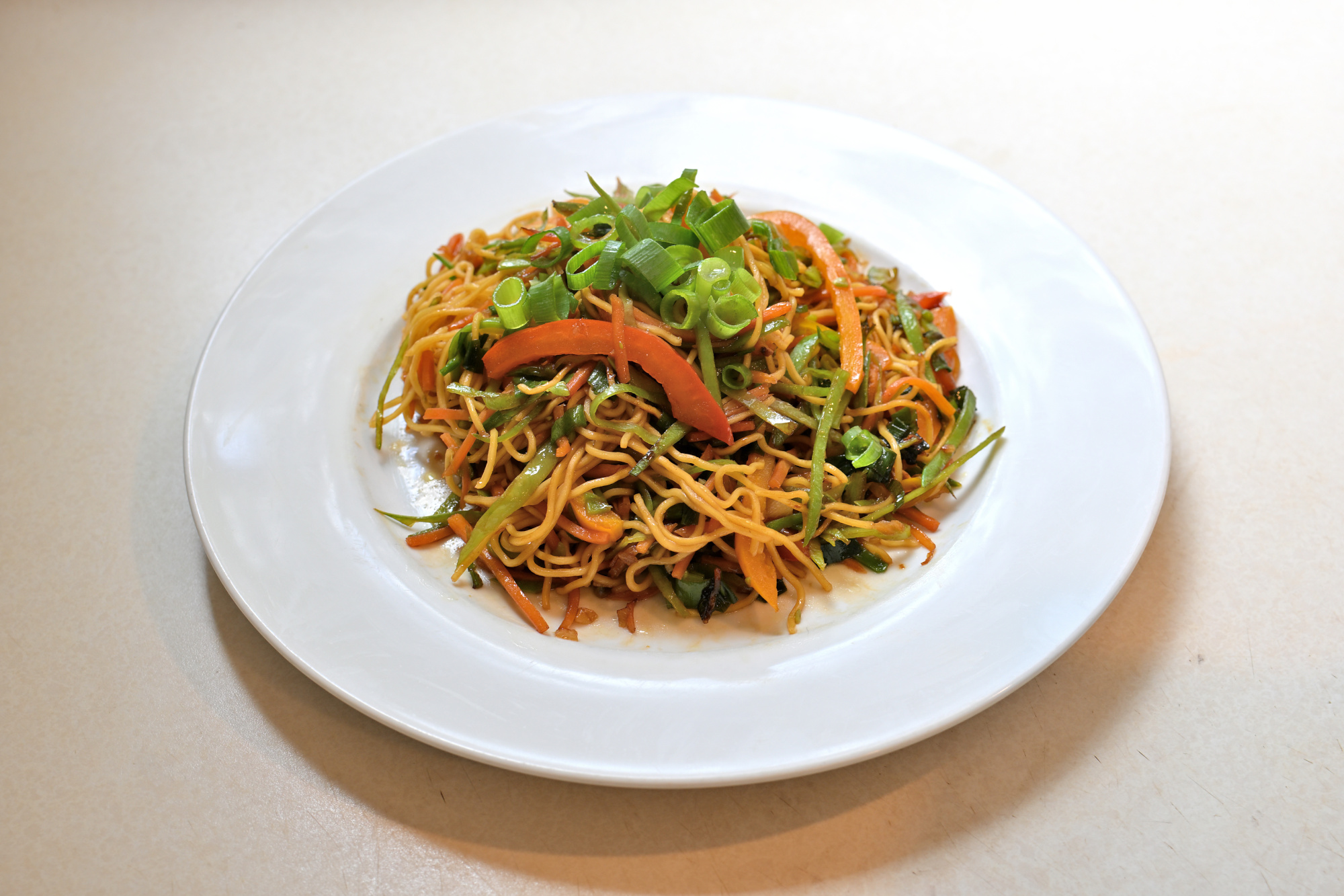
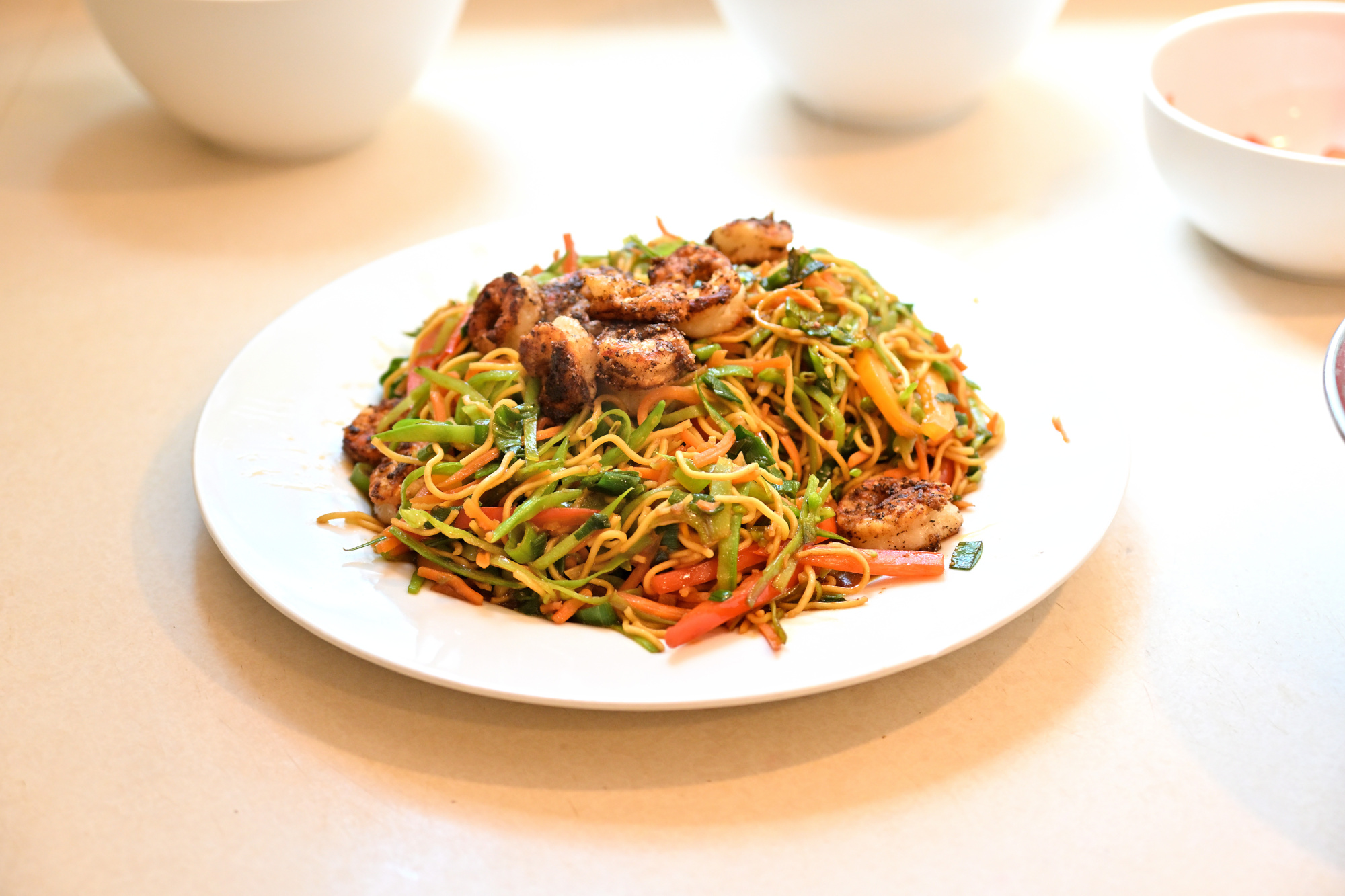
Auf dem Teller
Fertig. Ein Teller Chow Mein, frisch aus dem Wok, heiß, würzig und genau richtig für einen Beitrag, der ausnahmsweise nicht von Technik handelt. Wobei: Ein gutes Ergebnis nach sauberer Vorbereitung ist am Ende doch wieder ziemlich vertraut.
1/40s f/5 ISO 100/21° 16-50mm f/2,8 VR f=33mm/49mm
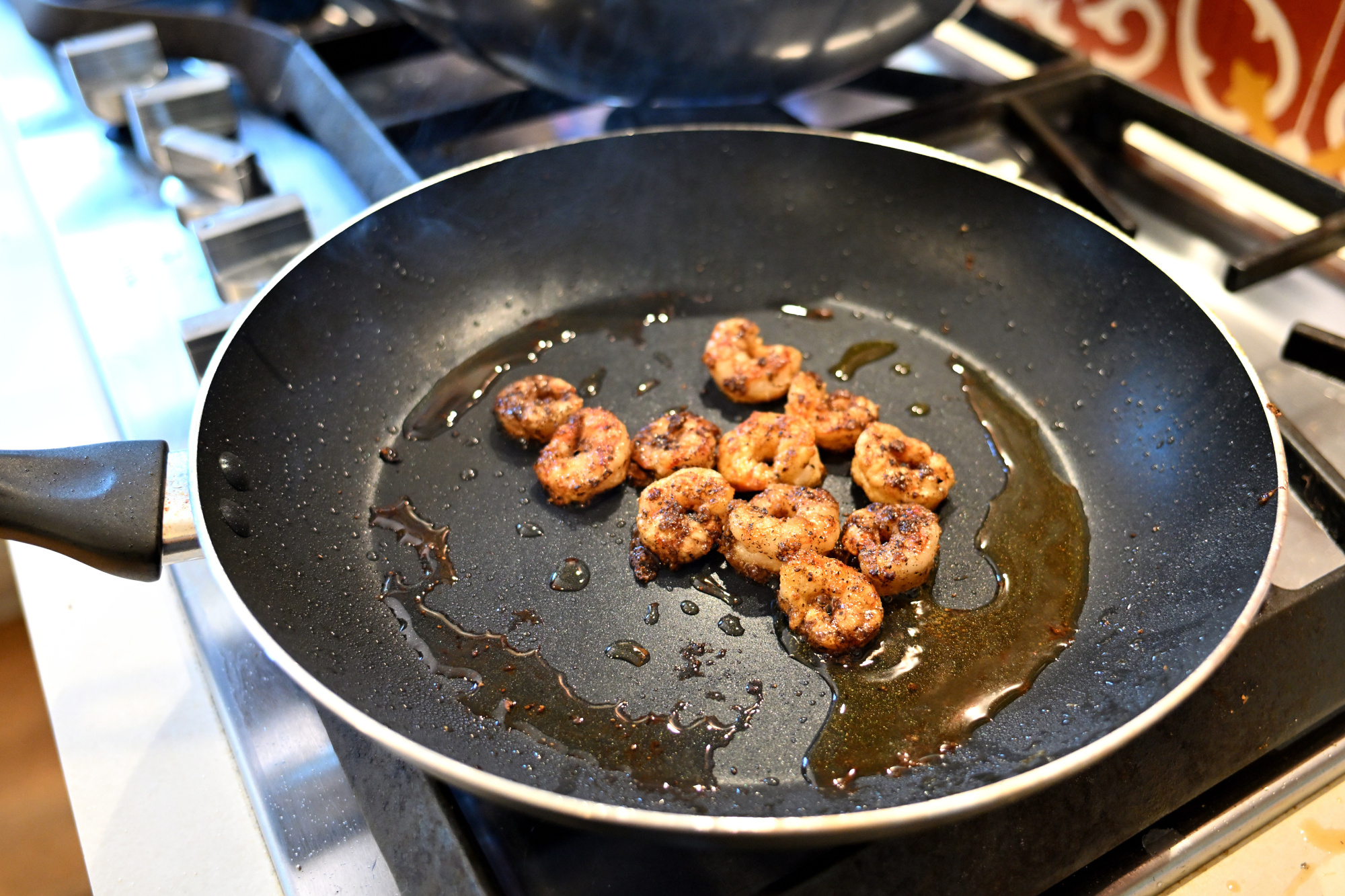
Mit Garnelen
Eine Variante, die dem Gericht nochmal eine etwas andere Richtung gibt. Die Garnelen passen sehr gut zu den gebratenen Nudeln und bringen noch einmal ihren eigenen Charakter mit.
1/125s f/2,8 ISO 1250/32° 16-50mm f/2,8 VR f=22mm/33mm
Fertig angerichtet
Am Teller sieht man dann, wie gut alles zusammenkommt: Farbe, Struktur und genau die Mischung aus Wok-Aroma und frischen Zutaten, die so ein Gericht ausmacht.
1/250s f/2,8 ISO 400/27° 16-50mm f/2,8 VR f=41mm/61mm
-
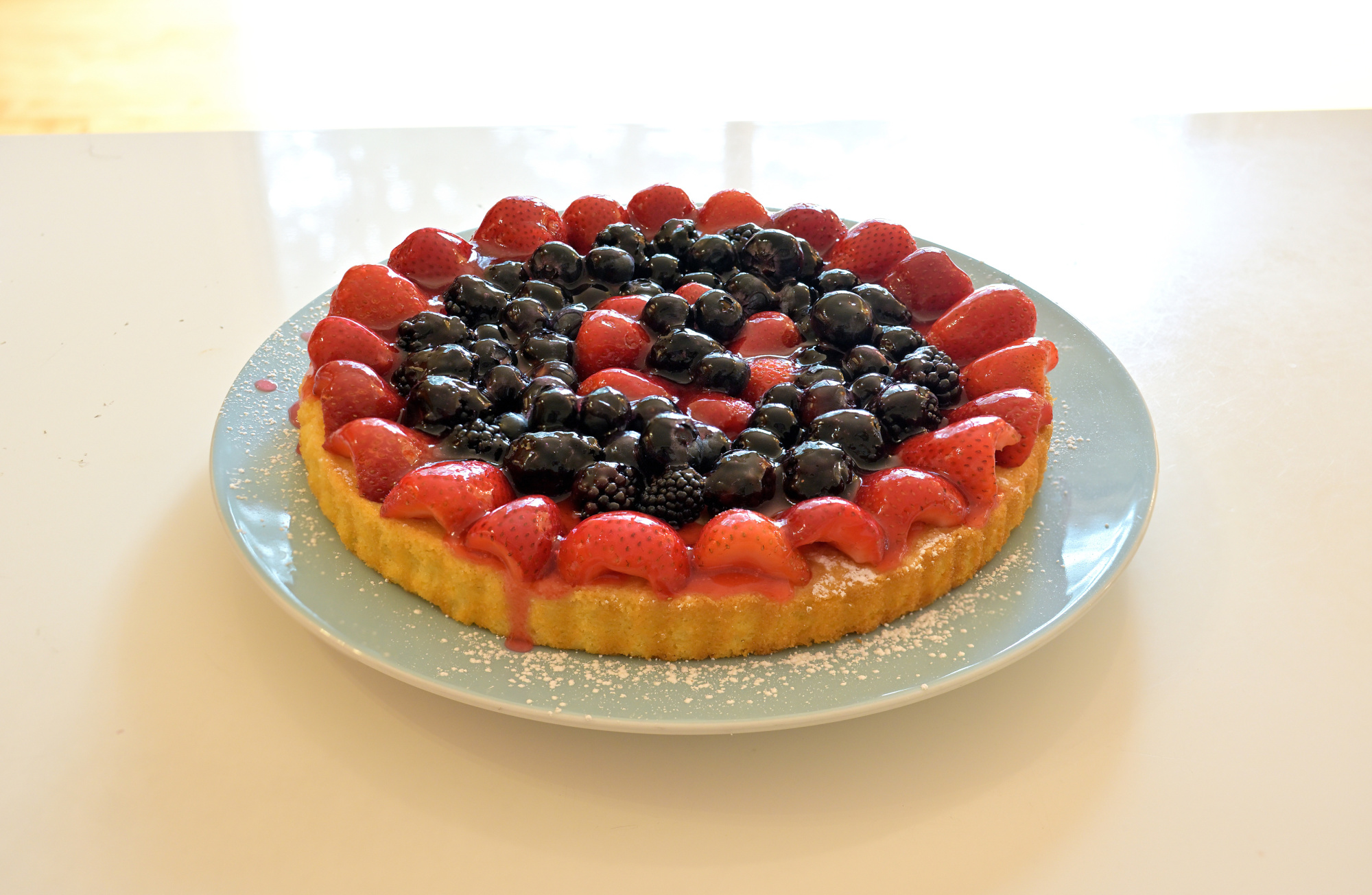
Obstkuchen zum Sonntagskaffee 🫐🍓
Sonntagskaffee und ein Obstkuchen mit Erdbeeren, Brombeeren und Blaubeeren.
Der Beerenmix wirkt auf dem Foto genauso gut wie auf dem Teller. Das Erdbeerrot setzt den Akzent, die dunklen Beeren bringen Tiefe, und die Struktur des Kuchenbodens hält das Bild zusammen. Genau so ein Motiv, das man gern etwas länger anschaut.
1/30s f/4 ISO 250/25°
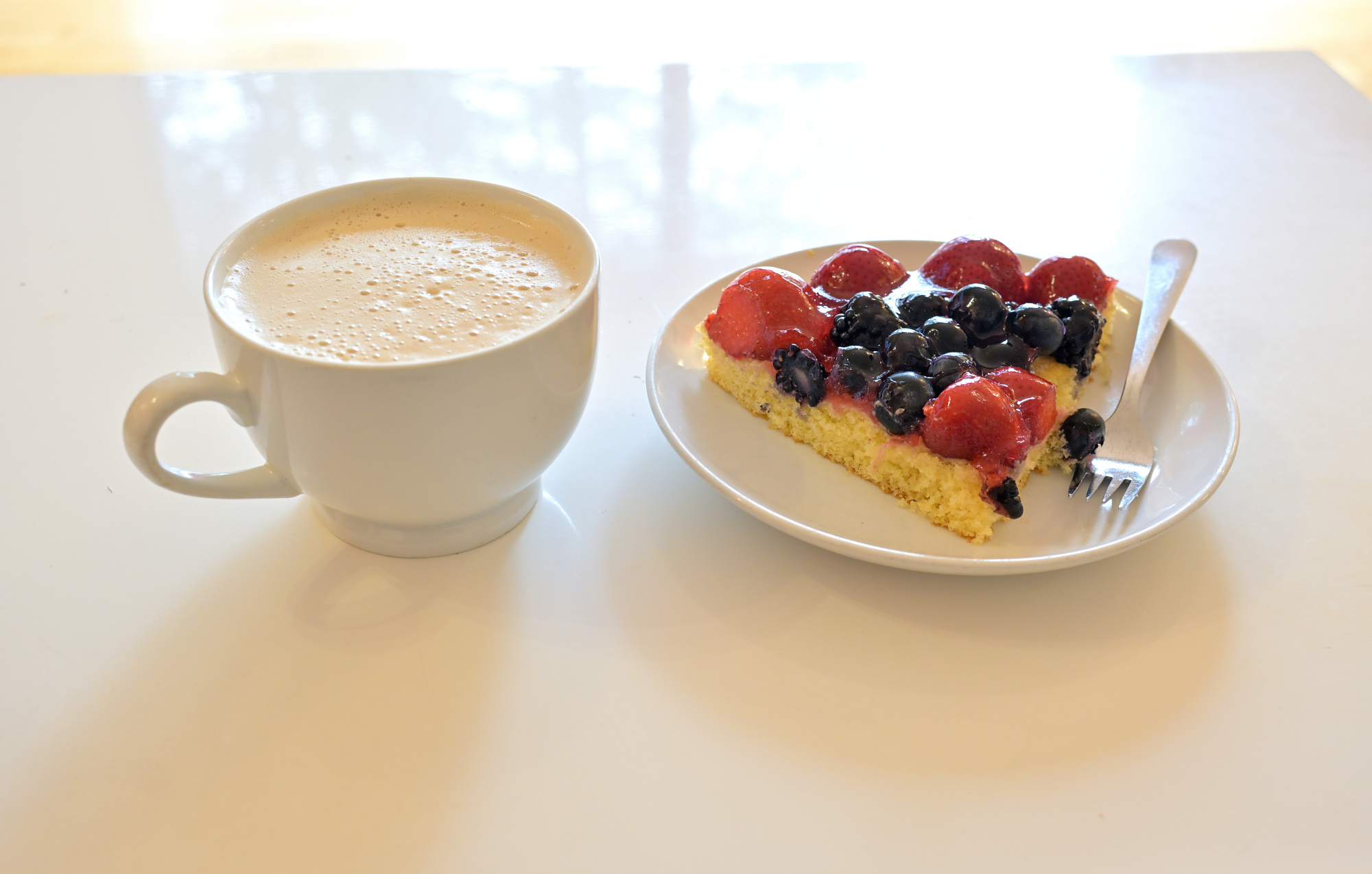
Dazu gehört natürlich auch ein Kaffee.
1/30s f/4 ISO 250/25° 16-50mm f/2,8 VR f=27mm/40mm
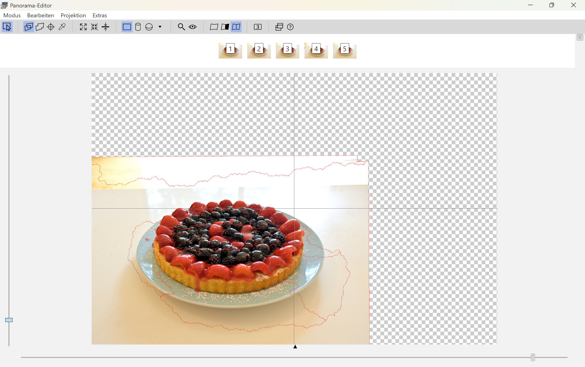
Wie das Bild entstanden ist: Fokus-Stacking mit 5 Aufnahmen
Damit die Details von vorne bis hinten scharf sind, habe ich das Kuchenfoto als Fokus-Stack aufgenommen. Dafür habe ich fünf Aufnahmen gemacht, jeweils mit einem anderen Fokuspunkt, also unterschiedlichen Schärfeebenen. So lässt sich die Schärfe gezielt über das Motiv verteilen, ohne dass man die Blende extrem schließen muss oder unnötig lange Belichtungszeiten riskiert.
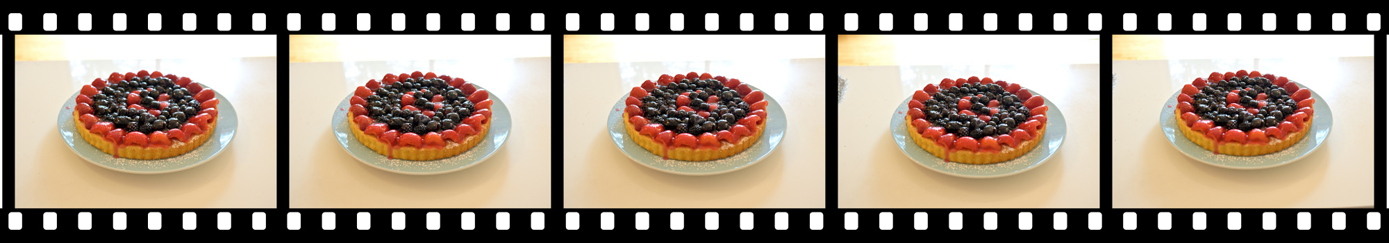
Anschließend habe ich die Serie in PTGui zusammengesetzt. Das Programm richtet die Einzelbilder sauber aus und überlagert sie. Am Ende entsteht ein Foto, das über die ganze Tiefe hinweg klar wirkt.
Im PTGui-Screenshot sieht man, wie die fünf Aufnahmen übereinander ausgerichtet sind. So entsteht daraus das durchgehend scharfe Bild.
Siehe Combine pictures with PTGui, Focus stacking
Ein reproduzierbares Experiment. Engpässe beim Versuchskuchen waren nicht zu erwarten.

-
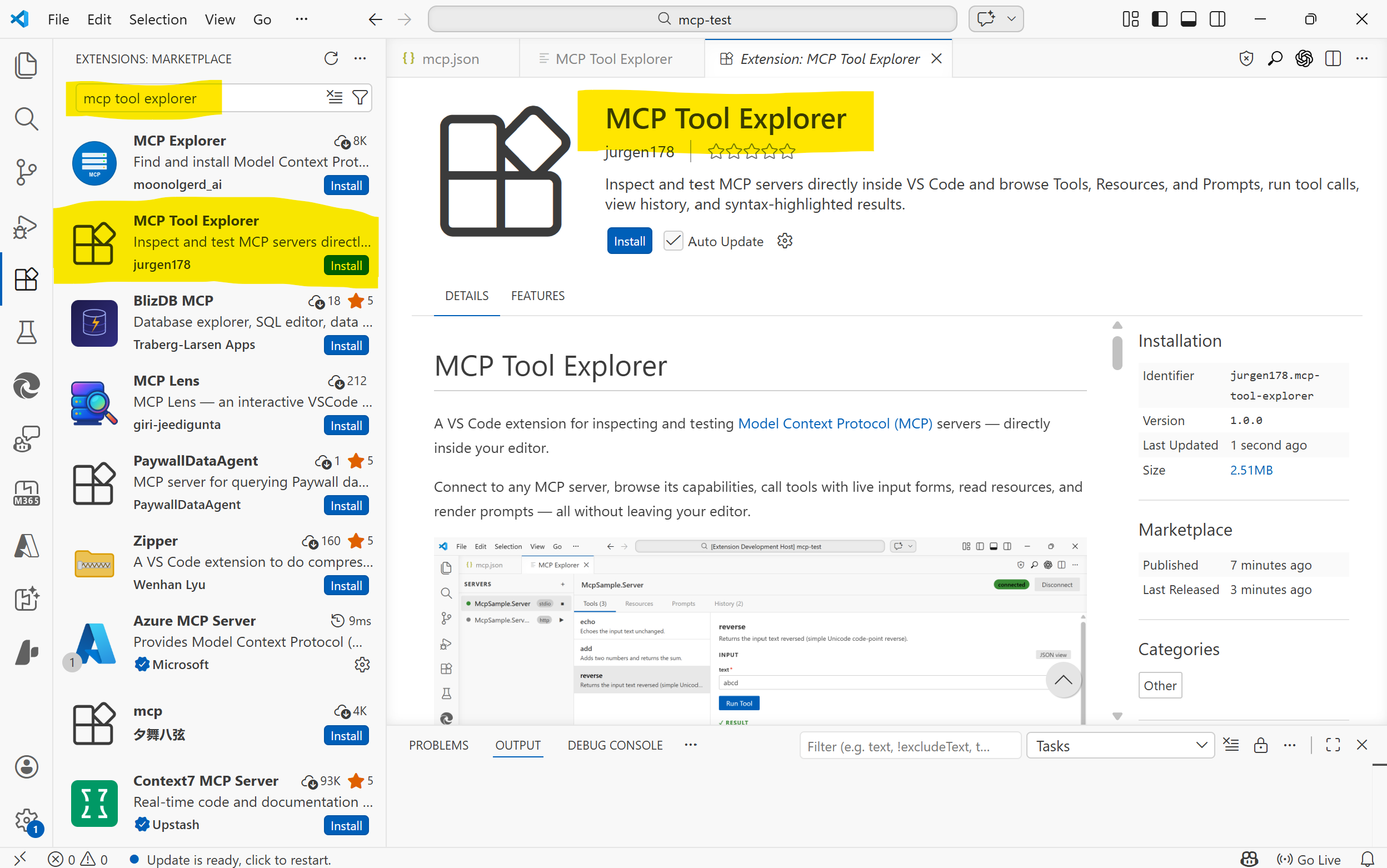
MCP Tool Explorer
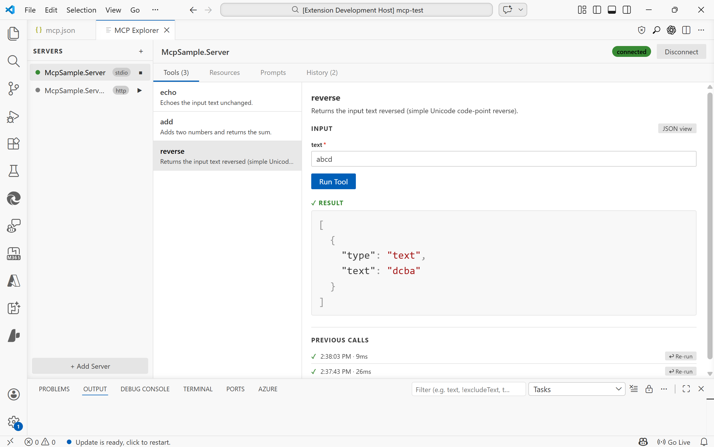
To work with Model Context Protocol (MCP) servers, I created a VS Code extension for inspecting and testing.
This extension connects to any MCP server, browse its capabilities, call tools with live input forms, read resources, render prompts, inspect notifications, and review connection traffic. All without leaving your editor.
Supports MCP Apps: tools that ship an interactive UI rendered directly inside the explorer.
https://github.com/jurgen178/mcp-tool-explorer
Features
Server Management
- Auto-discovery: automatically finds servers defined in
.vscode/mcp.jsonor themcp.serversworkspace setting - Manual registration: add any server on the fly via the Add Server dialog
- All three transports:
stdio,SSE, andStreamable HTTP - Capability indicators: each connected server shows T / R / P badges: green = items available, dimmed = declared but empty, hidden = not supported
Tools
- Browse all tools exposed by a server with their descriptions and parameter schemas
- Form view: auto-generated input form with type-aware fields (text, number, boolean toggle, enum select), including nested object fields
- JSON view: write raw JSON arguments with live validation hints (missing required fields, unknown properties)
- Run tools and see syntax-highlighted results; press Ctrl+Enter to run without leaving the keyboard
- Filter: a search bar appears above the tool list when a server exposes 10 or more tools
- Previous calls: the last 6 calls per tool are shown inline with one-click re-run
- The first available tool is automatically selected when a server connects
MCP Apps
Tools can declare a
ui://resource URI in their_meta.ui.resourceUrifield (MCP spec 2026-01-26). When such a tool is called, the explorer loads its HTML UI in a sandboxed iframe directly below the result, with no browser, no external window.The iframe communicates with the MCP server through the explorer's built-in JSON-RPC 2.0 bridge: it can call
tools/callandresources/readback against the server in real time, enabling fully interactive experiences like live regex visualizers, fractal renderers, or code diff viewers.Tools with an MCP App UI are marked with an MCP App badge in the tool list.
Resources
- List all resources and read their contents
- Results rendered with syntax highlighting
- Filter: a search bar appears when a server exposes 10 or more resources
- Resource list updates can be refreshed automatically when the server emits
notifications/resources/list_changed
Prompts
- Browse and render prompts with argument input support
- Filter: a search bar appears when a server exposes 10 or more prompts
- Prompt list updates can be refreshed automatically when the server emits
notifications/prompts/list_changed
Notifications & Events
- A dedicated Events tab shows incoming server notifications such as logging messages, progress updates, resource updates, and list-change notifications
- Related notifications can be visually grouped when they originate from the same server-side activity
- Streamable HTTP servers can surface server-initiated events, including out-of-band notifications over the standalone SSE stream
Saved Tests
- A dedicated Tests tab lets you save and replay tool calls as named test cases
- Organise tests into named groups
- Run individual tests or all tests in a group at once and see pass / fail results inline
- Tests are saved to
mcp-tests.jsonin the workspace root and automatically reloaded when the file changes - Supports both Form view and JSON view for test arguments; press Ctrl+Enter to run
Request History
- A dedicated History tab records every tool call, resource read, and prompt render
- See timestamp, duration, status (success / error), and expand to inspect the request arguments and response
- Re-run any past tool call directly from the timeline
Connection Diagnostics
- A dedicated Log tab records MCP transport activity for troubleshooting
- For HTTP-based servers, request and response details are captured to help diagnose initialization, fallback, auth, and notification-delivery issues
- Actionable hints are shown for common errors (host not found, connection refused, TLS issues, HTTP 4xx/5xx, invalid URL scheme)
- HTML error pages (e.g. IIS error responses) are automatically stripped to show only the relevant title
- In-progress connections can be cancelled at any time with the Cancel button
JSON Viewer
- Syntax-highlighted JSON output (keys, strings, numbers, booleans, nulls each in distinct colours)
- Copy to clipboard button appears on hover over any result
Getting Started
Installation
Install from the VS Code Marketplace, or build from source (see Building).
Test Server
If you want to try the extension against a ready-made MCP server, see mcp-test-server. It is useful for quickly validating tool calls, resources, and prompts while testing the explorer. A publicly reachable test endpoint is also available at https://bitfabrik.io/mcp.
Opening the Explorer
- Run
MCP: Open MCP Tool Explorerfrom the Command Palette (Ctrl+Shift+P)
Auto-discovery
If your workspace has a
.vscode/mcp.jsonfile, servers are discovered automatically when the extension activates. Example:{ "servers": { "my-stdio-server": { "type": "stdio", "command": "node", "args": ["./server/index.js"] }, "my-http-server": { "type": "http", "url": "http://localhost:3000/mcp" } } }Adding a Server Manually
Click + Add Server in the sidebar and fill in the connection details:
- stdio servers support
command,args(quote arguments that contain spaces),env, and an optional working directory (cwd) - HTTP / SSE servers support a
urland optional requestheaders
Manually added servers persist for the lifetime of the VS Code window.
Transports
Type Config key Description stdiocommand,args,env,cwdSpawns a local process httpurl,headersStreamable HTTP (MCP 2025-03 spec) sseurl,headersServer-Sent Events (legacy) For
stdioservers, the working directory defaults to the workspace root so relative paths incommandresolve correctly.
Building
# Install dependencies
npm install

# Build (webview + extension)
npm run build
The webview is a Vite + React app located in
webview-ui/. Runningnpm run buildat the root builds both the webview and the extension host automatically.
Project Structure
src/
  extension.ts              # Extension entry point
  types.ts                  # Extension-side types
  mcp/
    McpClientManager.ts     # MCP client connections (all transports)
    McpConfigDiscovery.ts   # Server auto-discovery
  panels/
    McpToolExplorerPanel.ts # WebView panel & message bridge
webview-ui/
  src/
    App.tsx                 # Root component & state management
    components/
      Sidebar.tsx           # Server list & connection controls
      ToolsPanel.tsx        # Tools tab
      ResourcesPanel.tsx    # Resources tab
      PromptsPanel.tsx      # Prompts tab
      EventsPanel.tsx       # Notifications and events tab
      HistoryPanel.tsx      # History timeline tab
      ConnectionLogPanel.tsx # Transport and connection log tab
      JsonViewer.tsx        # Syntax-highlighted JSON renderer
      AddServerModal.tsx    # Add Server dialog
Requirements
- VS Code 1.85 or later
- Node.js 18+ (for building from source)
- Auto-discovery: automatically finds servers defined in
-
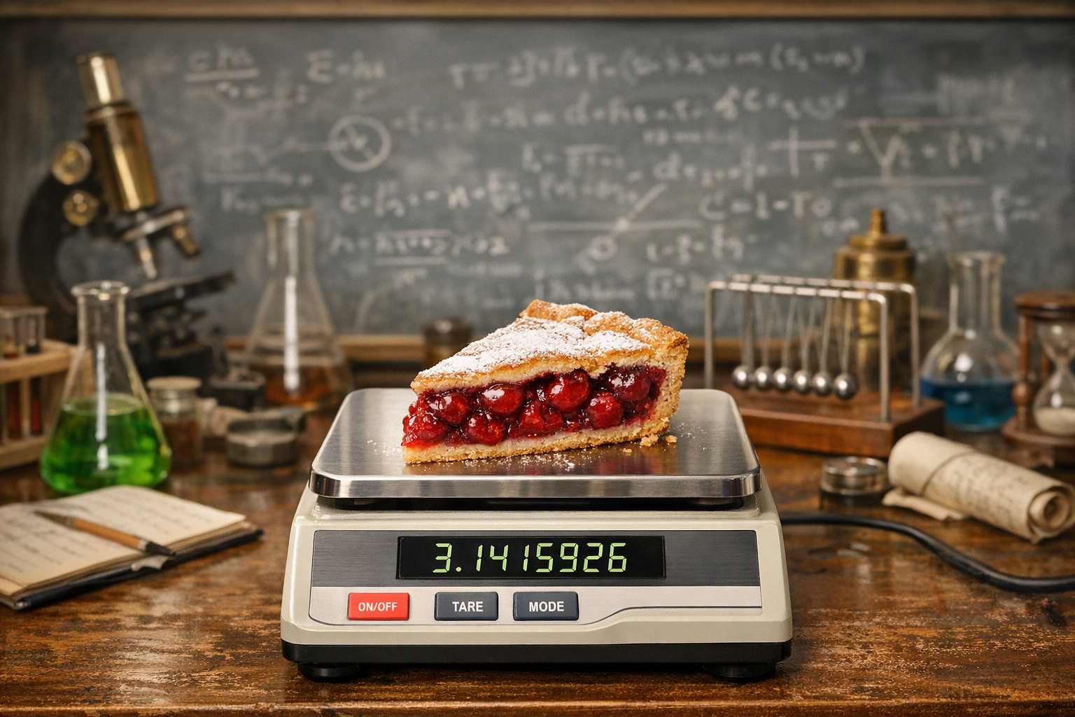
How Much Pi Do We Really Need
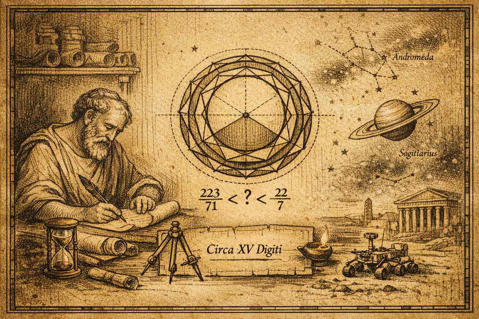
More than two thousand years ago, Archimedes2 tried to calculate the circumference of a circle. It was already known that larger circles have both a larger diameter and a larger circumference, but it was not clear whether the ratio between them would always remain the same.
By enclosing a circle between polygons with an increasing number of sides, he was able to show that this ratio is the same for every circle, and that its value can be bounded within steadily tightening intervals. Using a polygon of 96 sides, he proved that the value is contained in the interval
$$\frac{223}{71} < \pi < \frac{22}{7}$$
Archimedes narrowing the bounds
After Euler adopted the notation in 1736, the world denoted this value as $\pi$ 3
As an irrational number, its decimal expansion never repeats and never ends. And the search for more digits has never stopped.
This raises a simple question.
How many of those digits do we actually need to describe something real?
The circumference of a circle provides exactly that test.
The circumference of a circle is
$$C = \pi D$$
So any inaccuracy in $\pi$ directly affects the result.
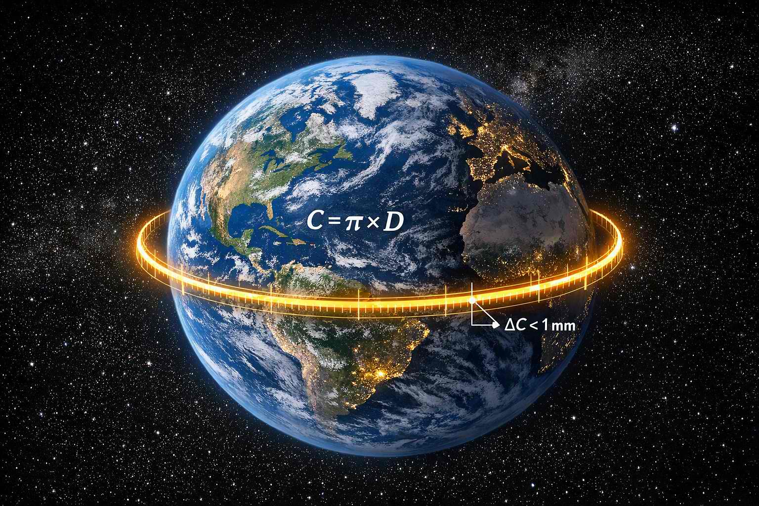
Example: The Earth
The diameter of the Earth is approximately
$$D_{Earth} \approx 12742\ km$$
We want the circumference to be correct within
$$1\ mm = 0.001\ m$$
This means the allowed error in the circumference is
$$\Delta C \leq 0.001\ m$$
Since
$$C = \pi D$$
any error in $\pi$ causes
$$\Delta C = D \cdot \Delta \pi$$
So the required accuracy of $\pi$ must satisfy
$$D \cdot \Delta \pi \leq 0.001$$
Solving for $\Delta \pi$ leads to
$$\Delta \pi \leq \frac{0.001}{12742\cdot1000}$$
$$\Delta \pi \leq 7.85 \times 10^{-11}$$
That corresponds to roughly 10 decimal places of $\pi$. Using 10 places results in an error of about $10^{-11}$, which is within the required bound.
So if you use
$$\pi_{10} = 3.1415926536$$
you can calculate the circumference of the entire Earth with an error smaller than one millimeter.
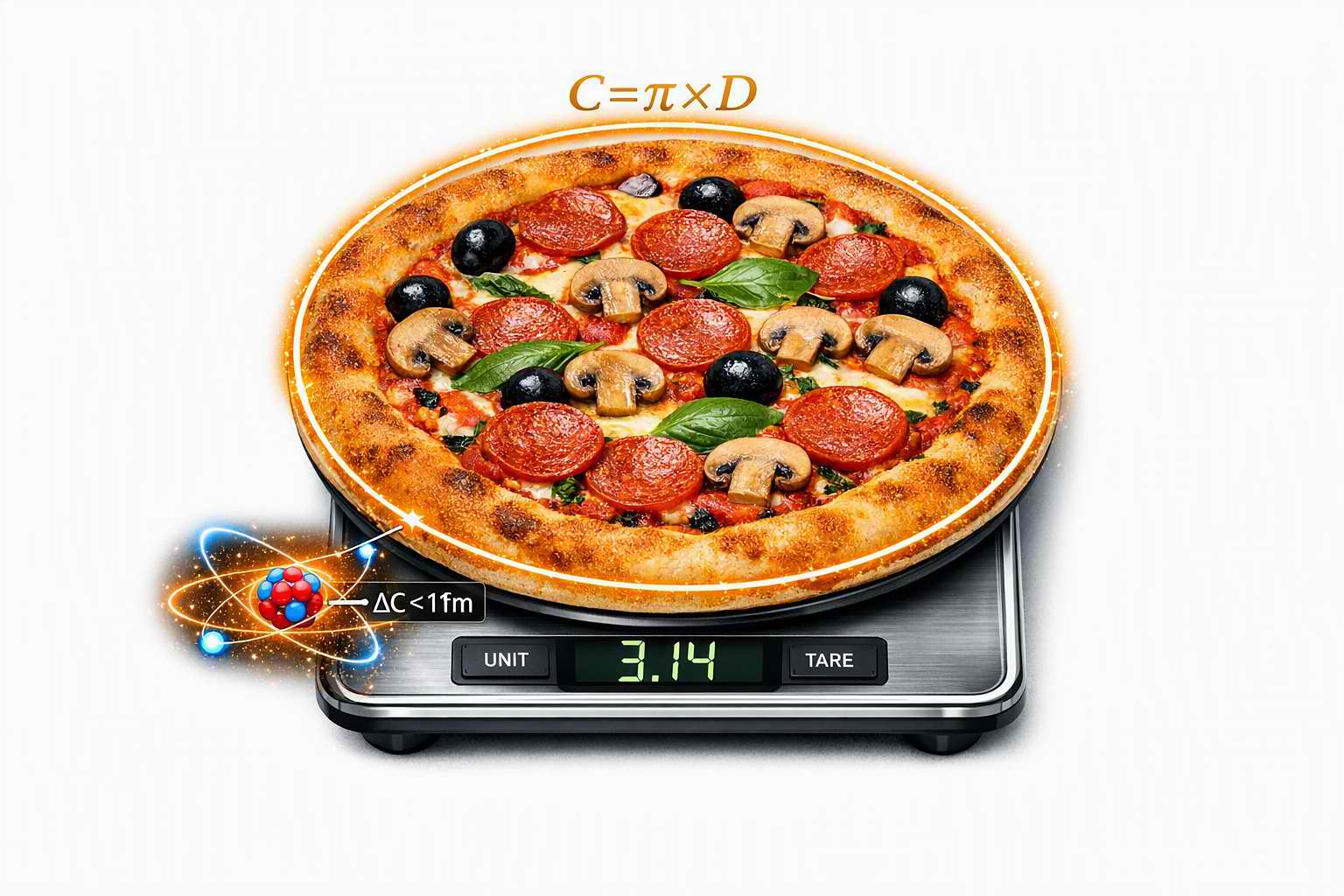
Example: A Pizza
The diameter of a pizza is approximately
$$D_{Pizza} \approx 0.30\ m$$
This time we set the target accuracy to the diameter of an atomic nucleus
$$1\ \text{fm} = 10^{-15}\ m$$
Applying the same formula leads to
$$\Delta \pi \leq \frac{10^{-15}}{0.30}$$
$$\Delta \pi \leq 3.3 \times 10^{-15}$$
That corresponds to roughly 15 decimal places of $\pi$.
So if you use
$$\pi_{15} = 3.141592653589793$$
you can calculate the circumference of a pizza with an error smaller than the diameter of an atomic nucleus.
Example: The Observable Universe
Now let us scale things up.
The diameter of the observable universe is estimated at roughly
$$D_{Universe} \approx 8.8 \times 10^{26}\ m$$
Using the same formula with a target accuracy of 1 mm, as in the Earth example, leads to
$$\Delta \pi \leq \frac{0.001}{8.8 \times 10^{26}}$$
$$\Delta \pi \leq 1.14 \times 10^{-30}$$
That corresponds to roughly 30 decimal places of $\pi$.
So if you use
$$\pi_{30} = 3.141592653589793238462643383279$$
you can calculate the circumference of the entire observable universe with an error smaller than one millimeter.

Conclusion
Ten digits of $\pi$ are enough for planetary scale.
Fifteen digits are enough to measure a pizza to the width of an atomic nucleus.
Thirty digits are enough for cosmic scale.
Beyond that, the digits describe no physical quantity we can measure, only the internal consistency of mathematics itself.
Fifteen digits are also exactly what NASA uses to navigate spacecraft across the solar system, the same precision that measures a pizza to the width of an atomic nucleus.
They have not yet missed a planet.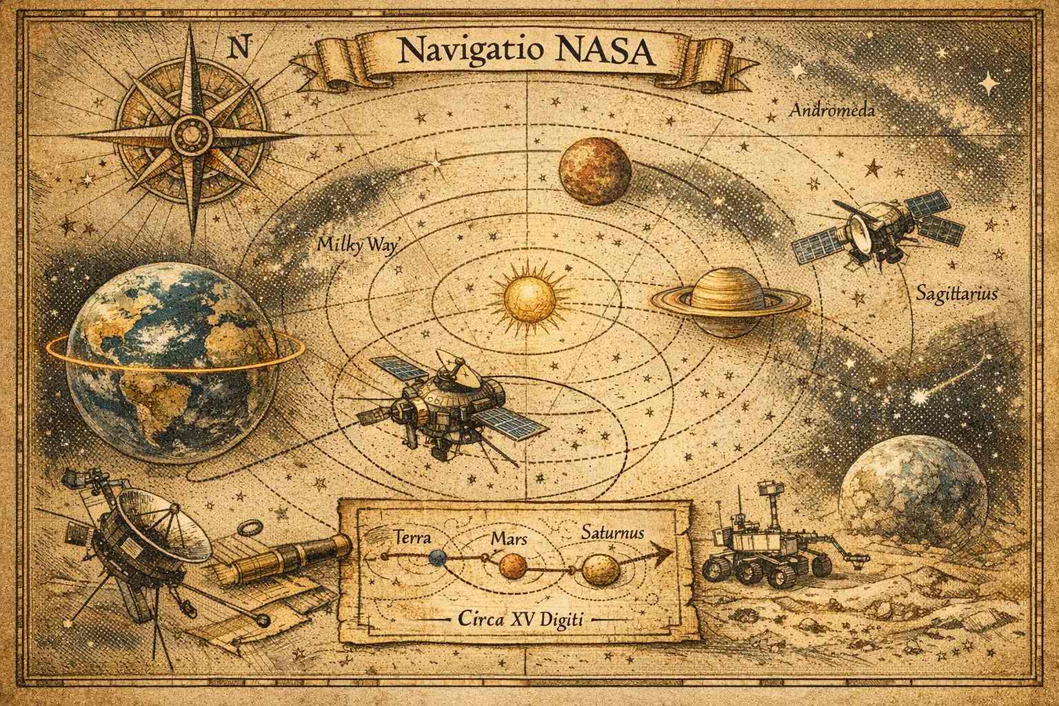
Interplanetary navigation with finite precision
See also Engineering Pi Day
-
The lab has seen many upgrades.
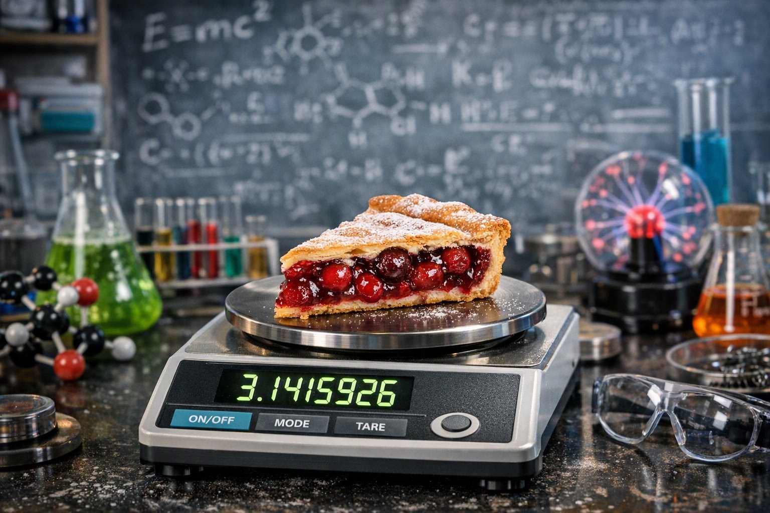
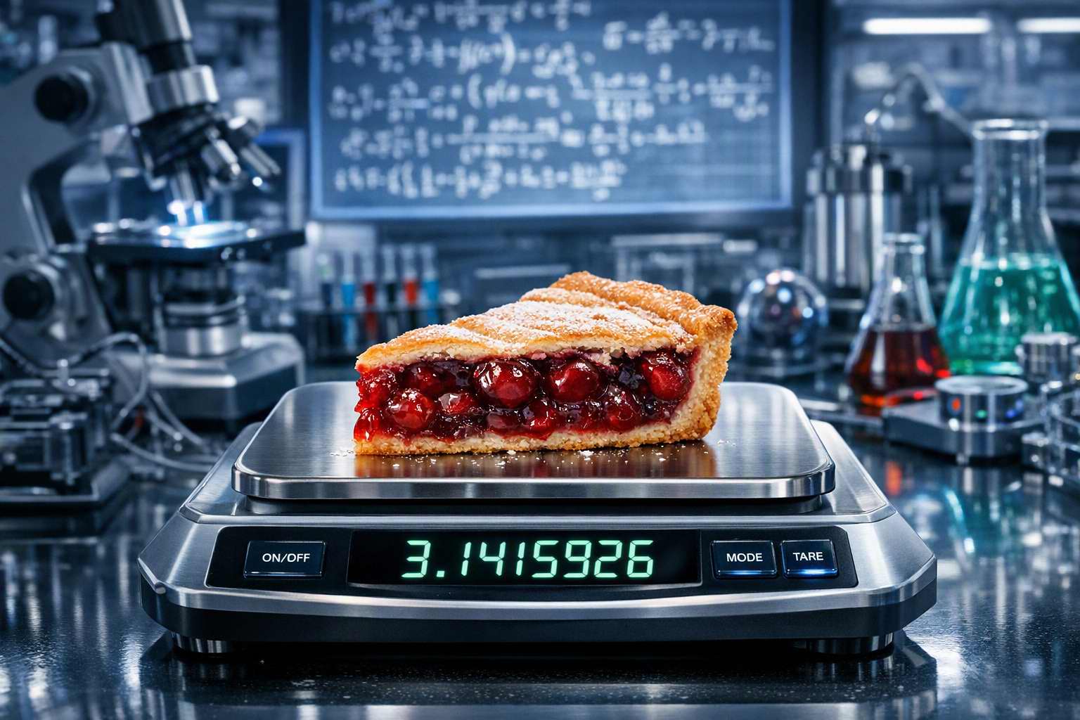
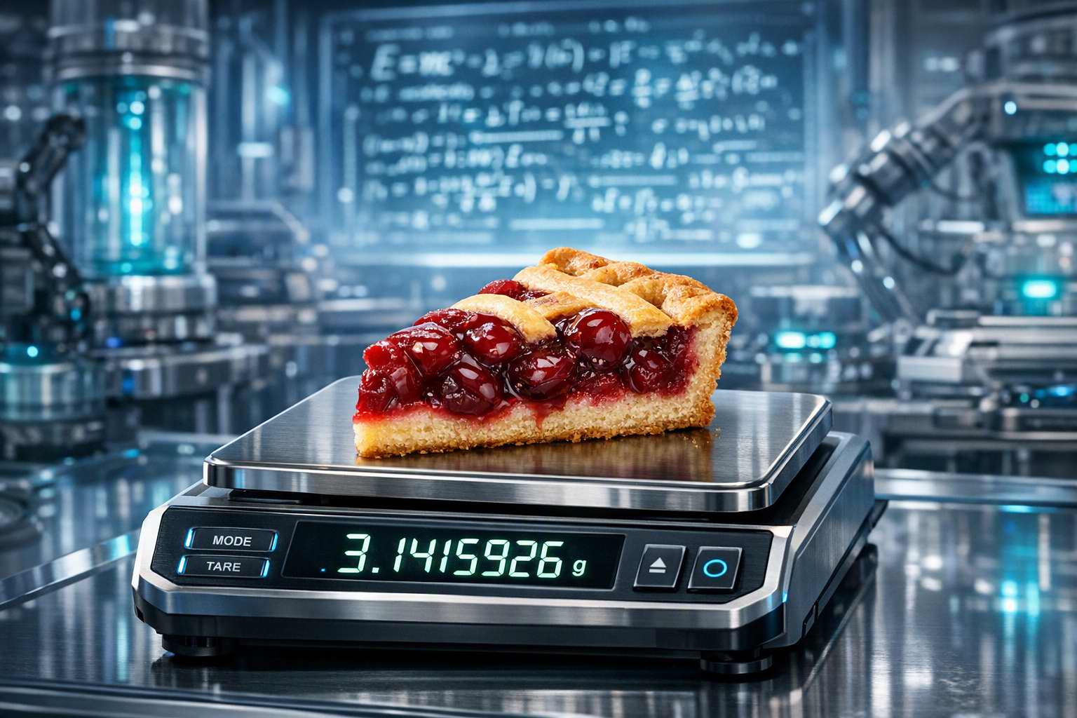 The Pie remained entirely indifferent.
Even they could not find a pattern.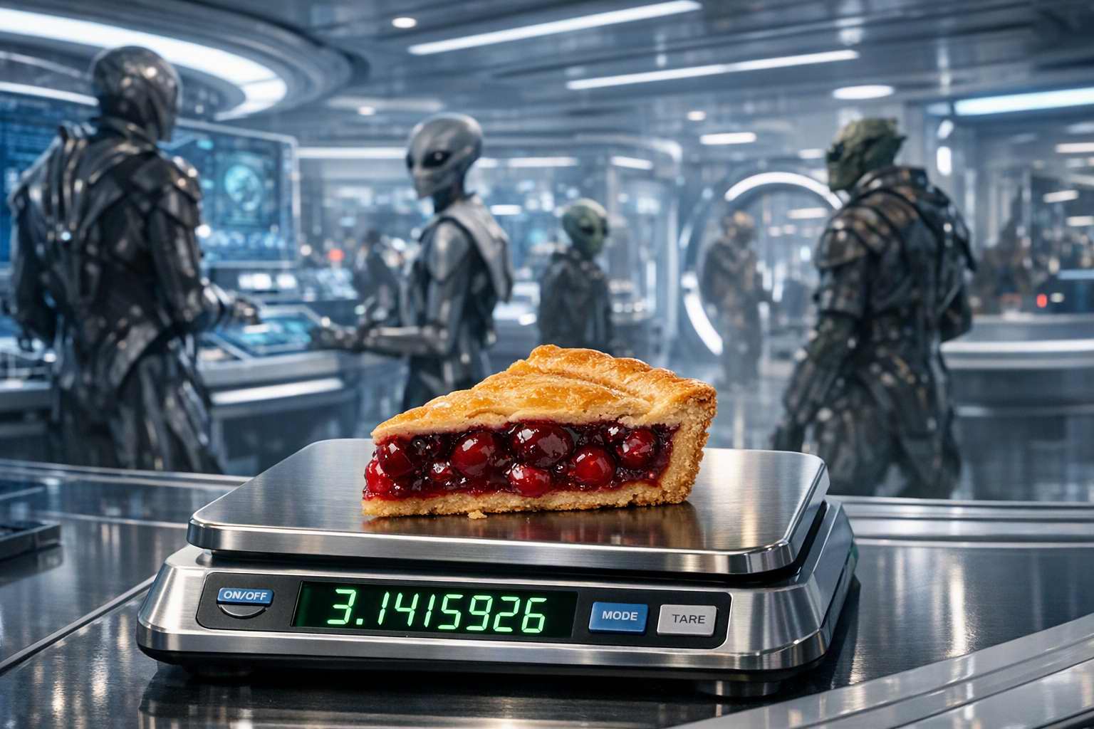
Archimedes' office, circa 250 BC. The Pie was already indifferent.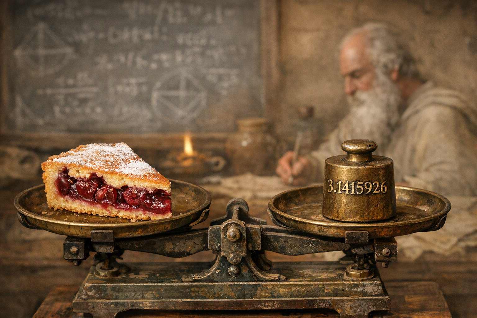 ↩
↩ -
Archimedes of Syracuse (c. 287-212 BC) derived his bounds on π in Measurement of a Circle. A result that stood as the standard approximation for centuries. ↩
-
$$\pi_{314}=3.14159265358979323846264338327950288419716939937510582097494459230781640628620899862803482534211706798214808651328230664709384460955058223172535940812848111745028410270193852110555964462294895493038196442881097566593344612847564823378678316527120190914564856692346034861045432664821339360726024914127372458700660631$$ ↩
-