-
A Cat at Dusk, ISO 12800
Not every improvement in technology needs a big explanation. Sometimes it is just there in a simple picture taken late in the day, when the light is already fading and everything feels a little softer.
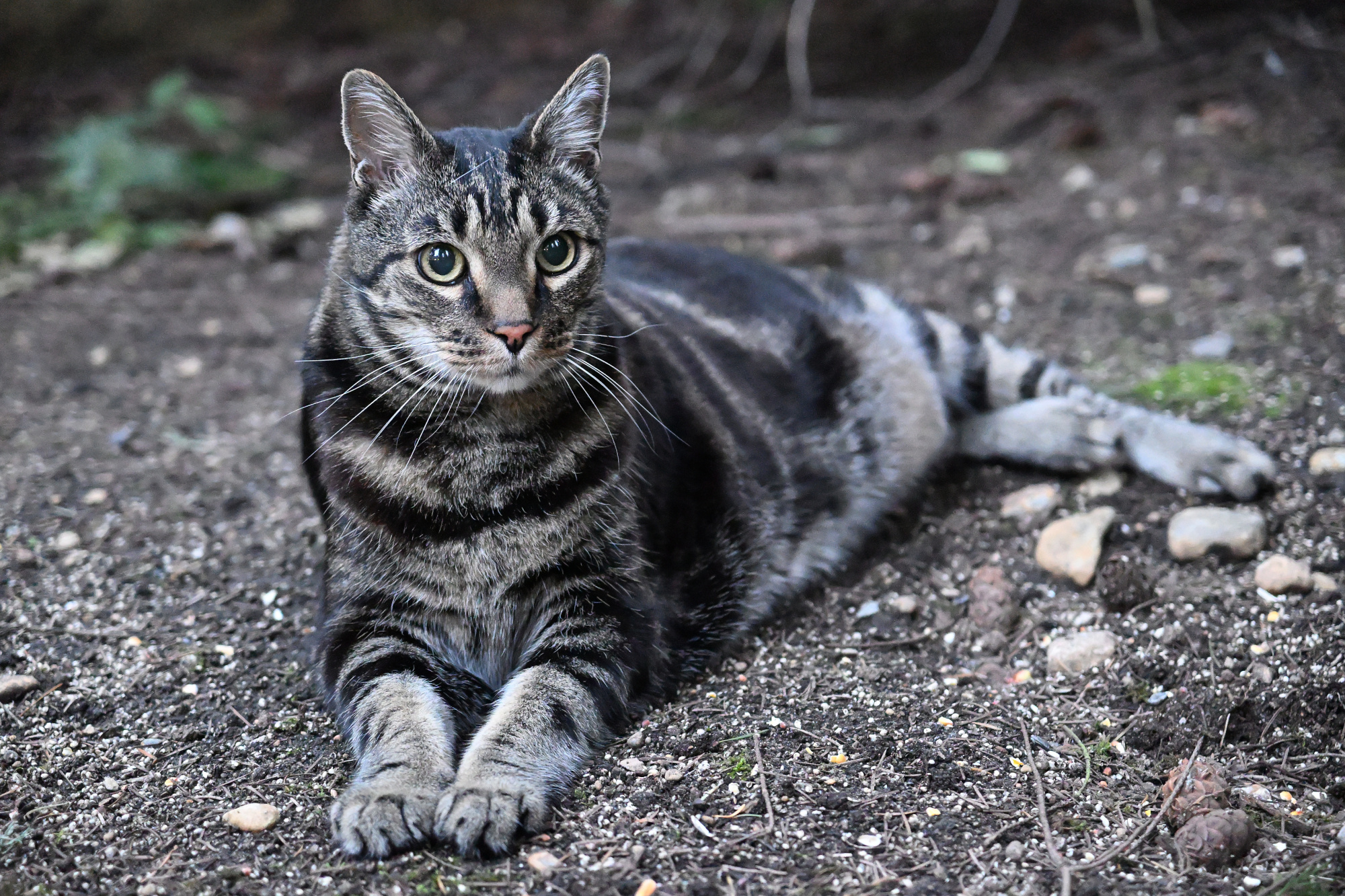
These two photos of our cat were taken at dusk with the Nikon Z50 at ISO 12800 and f/2.8. What I like about them is how calm and natural they feel. The images are sharp, the detail is there, and the whole scene keeps its quiet evening mood.
That is one of the nice things about modern cameras. They make this kind of picture easier and leave more room to focus on the subject, the light, and the moment.
Two quiet moments in the fading evening light
1/80s f/2,8 ISO 12800/42° 16-50mm f/2,8 VR f=50mm/75mm
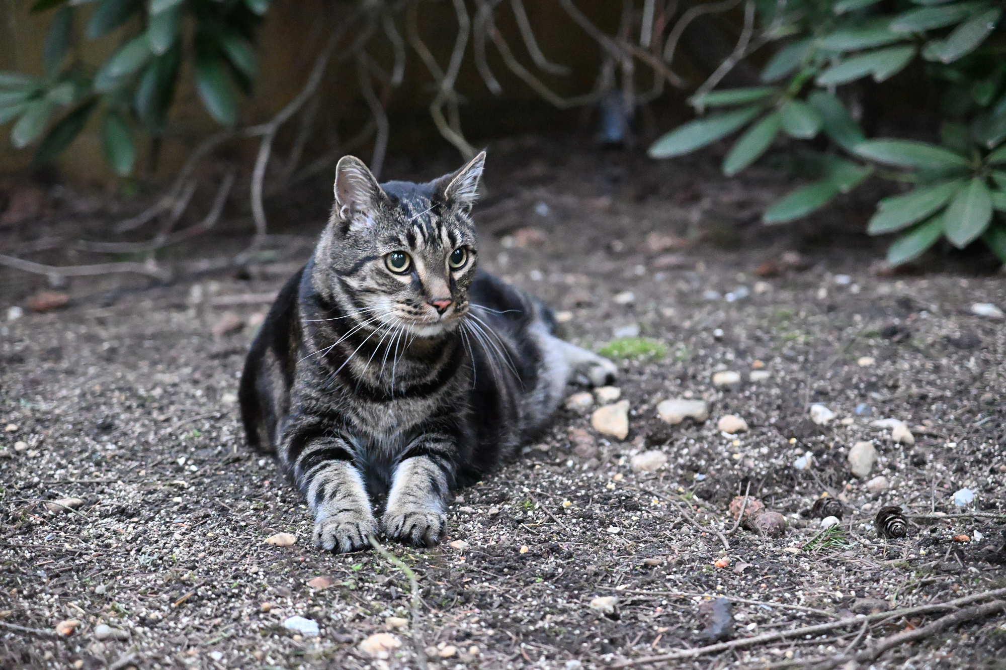
1/80s f/2,8 ISO 12800/42° 16-50mm f/2,8 VR f=50mm/75mm
A closer look at the detail, and a nice reminder of how well this works these days.
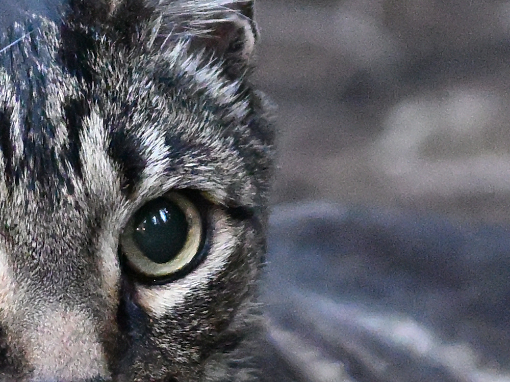
From the Z50 to JPEG for the web via Nikon NX Studio, with everything left at the default settings.
-
Obstkuchen zum Sonntagskaffee 🫐🍓
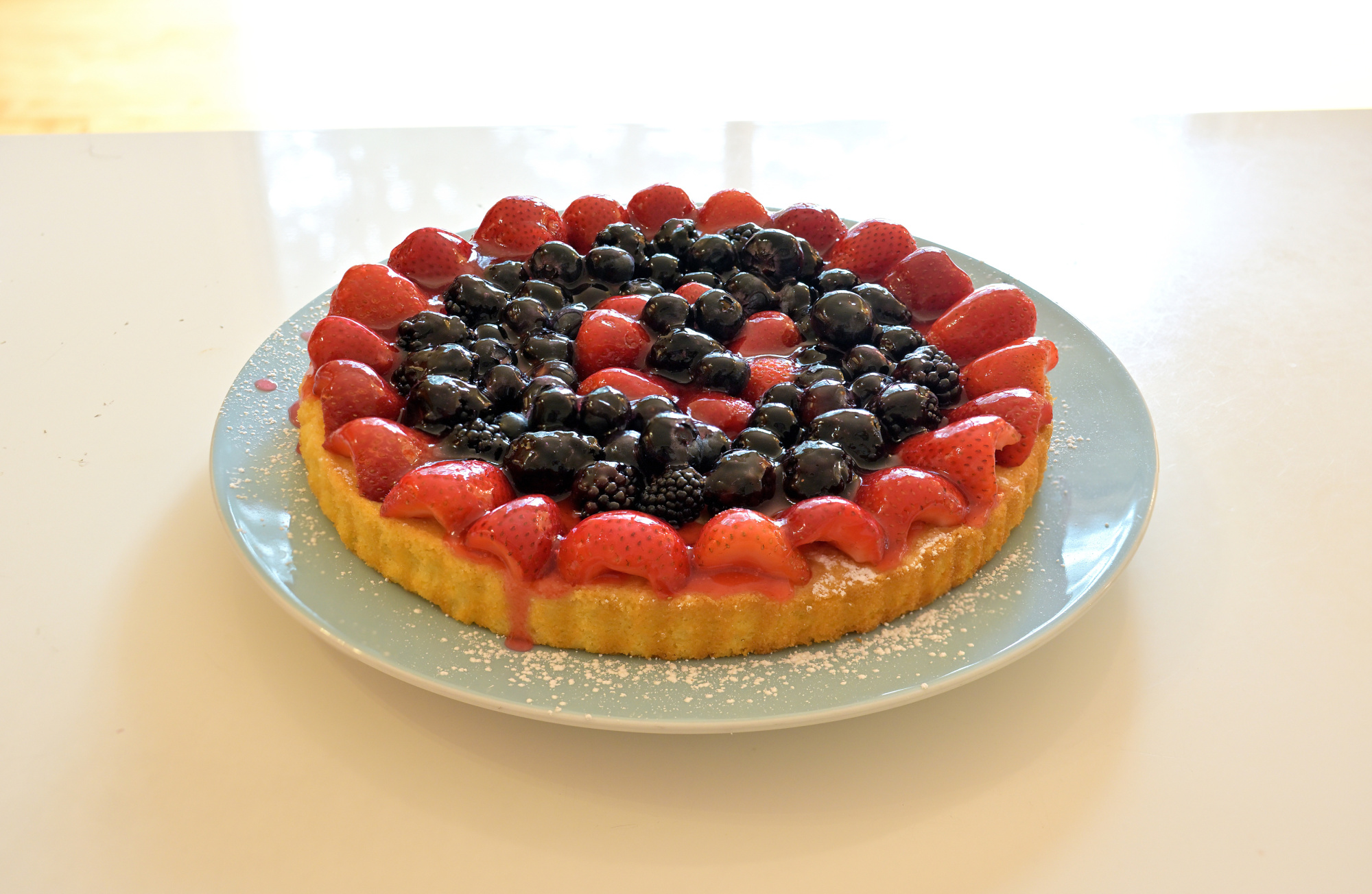
Sonntagskaffee und ein Obstkuchen mit Erdbeeren, Brombeeren und Blaubeeren.
Der Beerenmix wirkt auf dem Foto genauso gut wie auf dem Teller. Das Erdbeerrot setzt den Akzent, die dunklen Beeren bringen Tiefe, und die Struktur des Kuchenbodens hält das Bild zusammen. Genau so ein Motiv, das man gern etwas länger anschaut.
1/30s f/4 ISO 250/25°
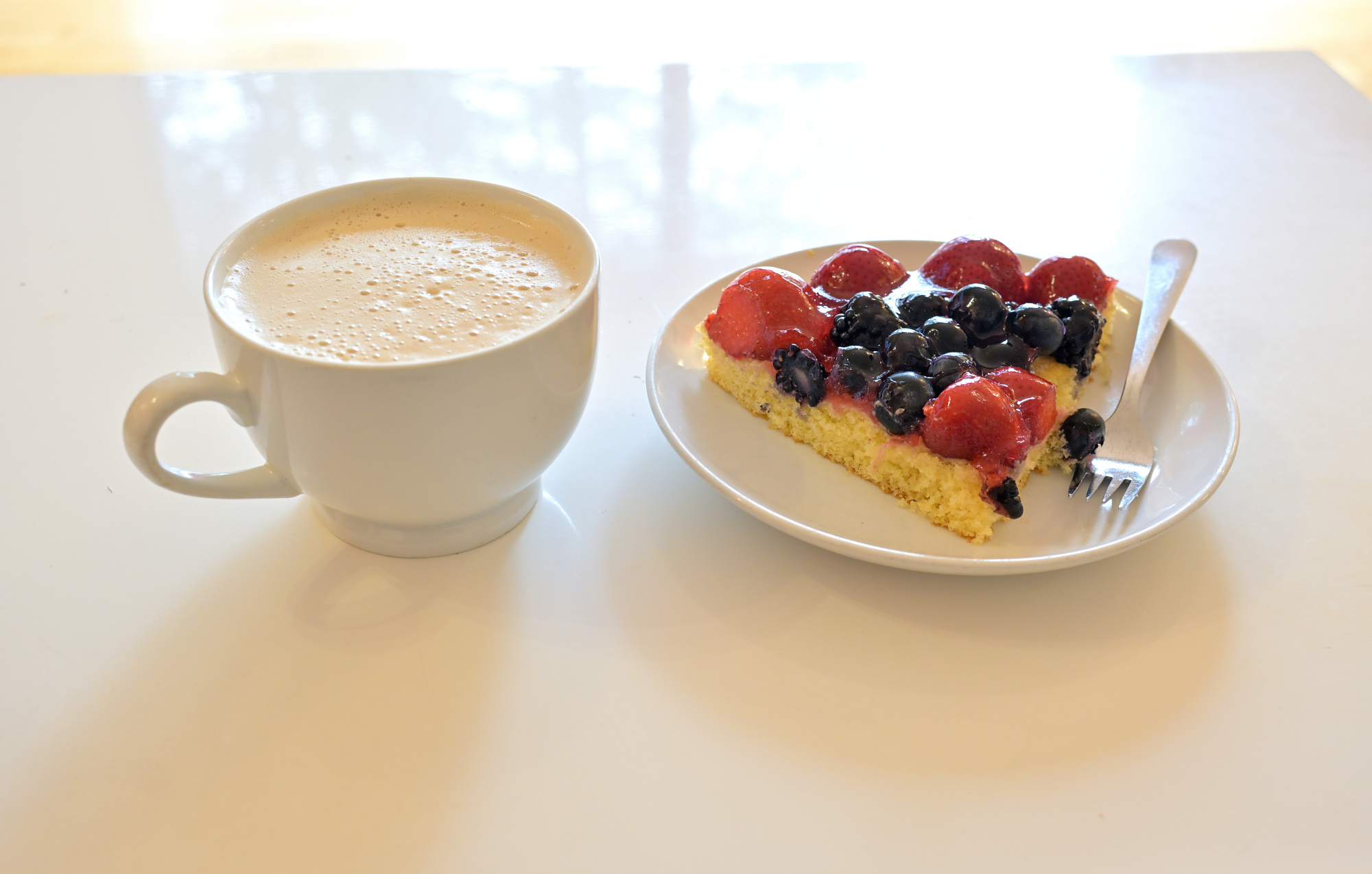
Dazu gehört natürlich auch ein Kaffee.
1/30s f/4 ISO 250/25° 16-50mm f/2,8 VR f=27mm/40mm
Wie das Bild entstanden ist: Fokus-Stacking mit 5 Aufnahmen
Damit die Details von vorne bis hinten scharf sind, habe ich das Kuchenfoto als Fokus-Stack aufgenommen. Dafür habe ich fünf Aufnahmen gemacht, jeweils mit einem anderen Fokuspunkt, also unterschiedlichen Schärfeebenen. So lässt sich die Schärfe gezielt über das Motiv verteilen, ohne dass man die Blende extrem schließen muss oder unnötig lange Belichtungszeiten riskiert.

Anschließend habe ich die Serie in PTGui zusammengesetzt. Das Programm richtet die Einzelbilder sauber aus und überlagert sie. Am Ende entsteht ein Foto, das über die ganze Tiefe hinweg klar wirkt.
Im PTGui-Screenshot sieht man, wie die fünf Aufnahmen übereinander ausgerichtet sind. So entsteht daraus das durchgehend scharfe Bild.
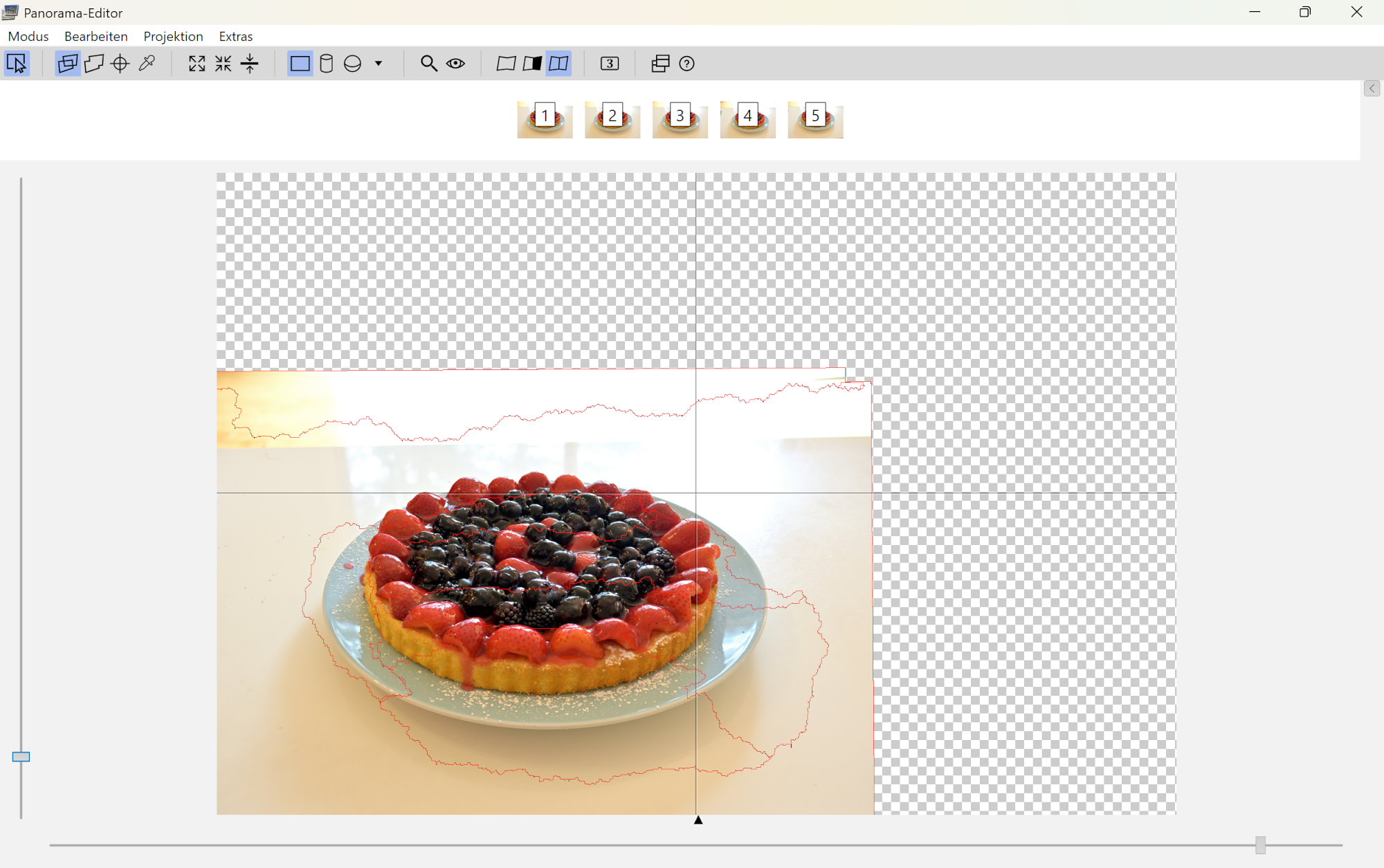
Siehe Combine pictures with PTGui, Focus stacking
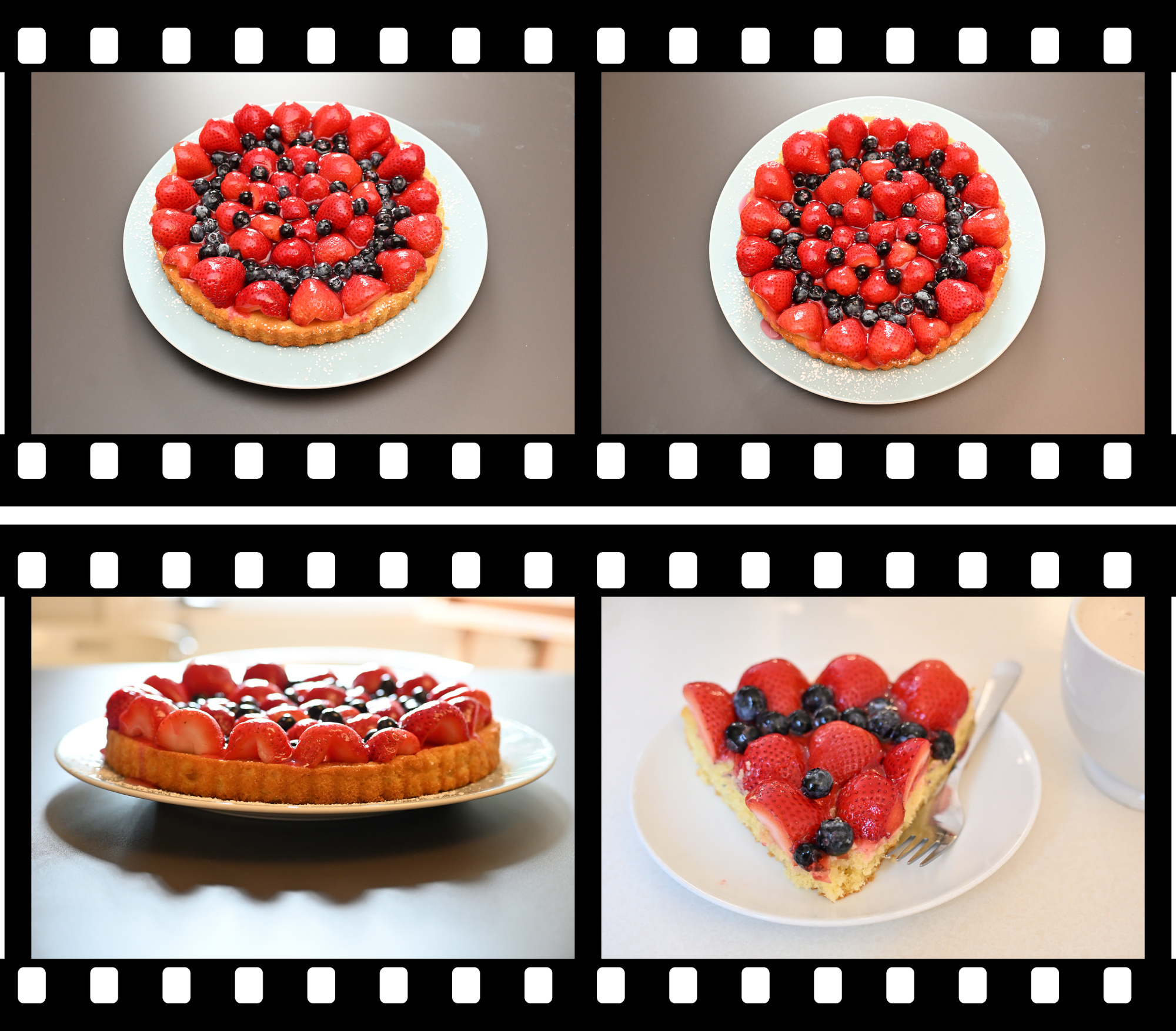
Ein reproduzierbares Experiment. Engpässe beim Versuchskuchen waren nicht zu erwarten.
-
Märzschnee
1/125s f/3,5 ISO 100/21° 16-50mm f/2,8 VR f=28mm/42mm
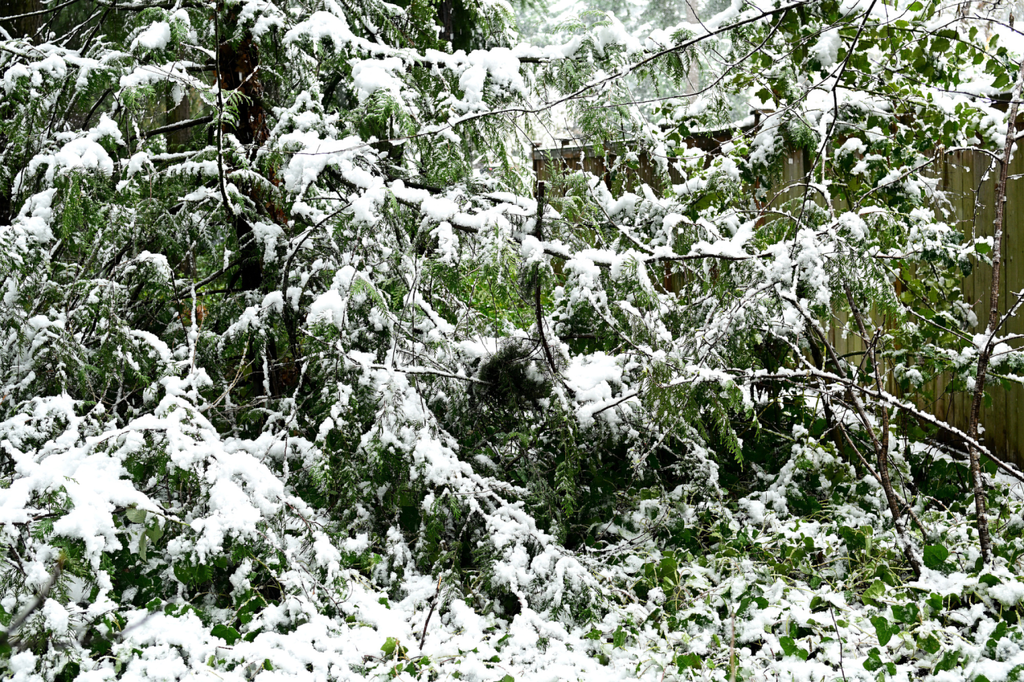
1/125s f/3,5 ISO 100/21° 16-50mm f/2,8 VR f=50mm/75mm
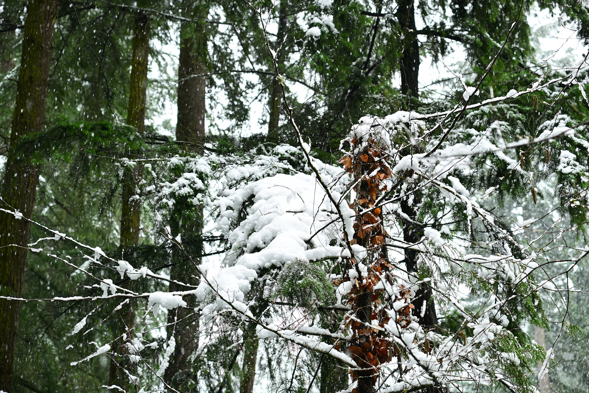
1/125s f/3,5 ISO 100/21° 16-50mm f/2,8 VR f=35mm/52mm
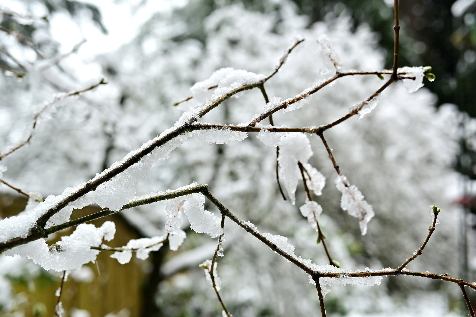
1/125s f/3,5 ISO 100/21° 16-50mm f/2,8 VR f=35mm/52mm
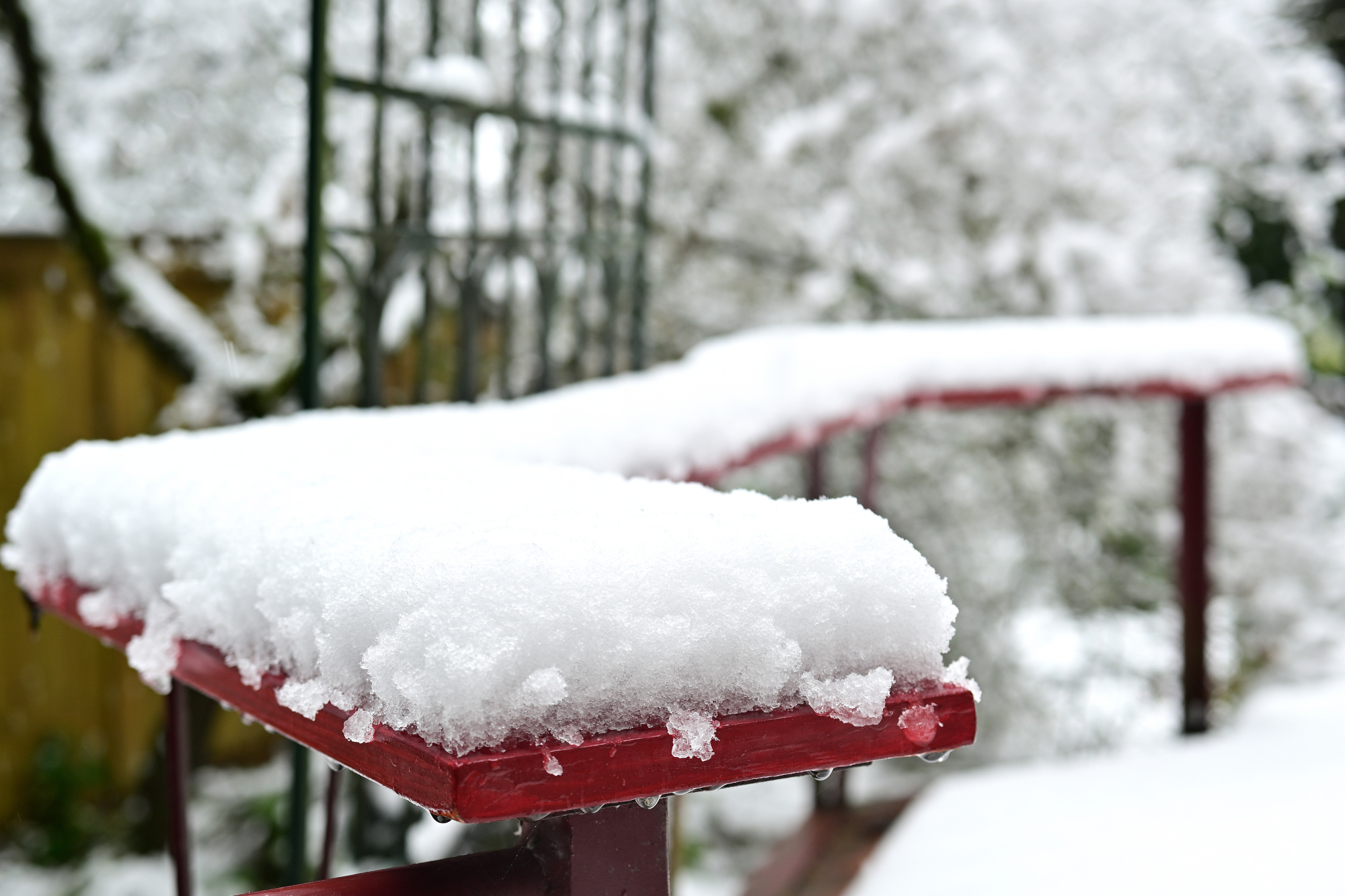
Lossless Minecraft Version
1/125s f/3,5 ISO 100/21° 16-50mm f/2,8 VR f=30mm/45mm
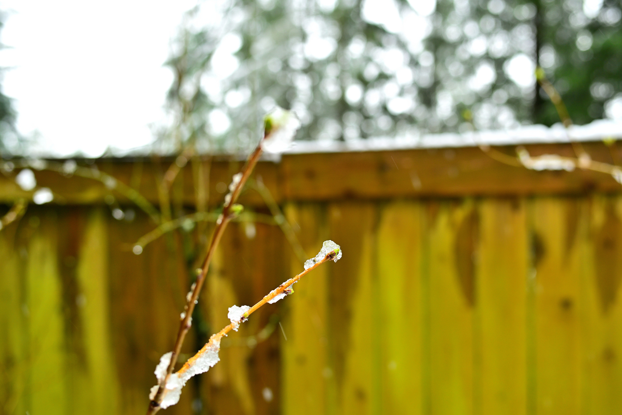
1/125s f/3,5 ISO 100/21° 16-50mm f/2,8 VR f=50mm/75mm
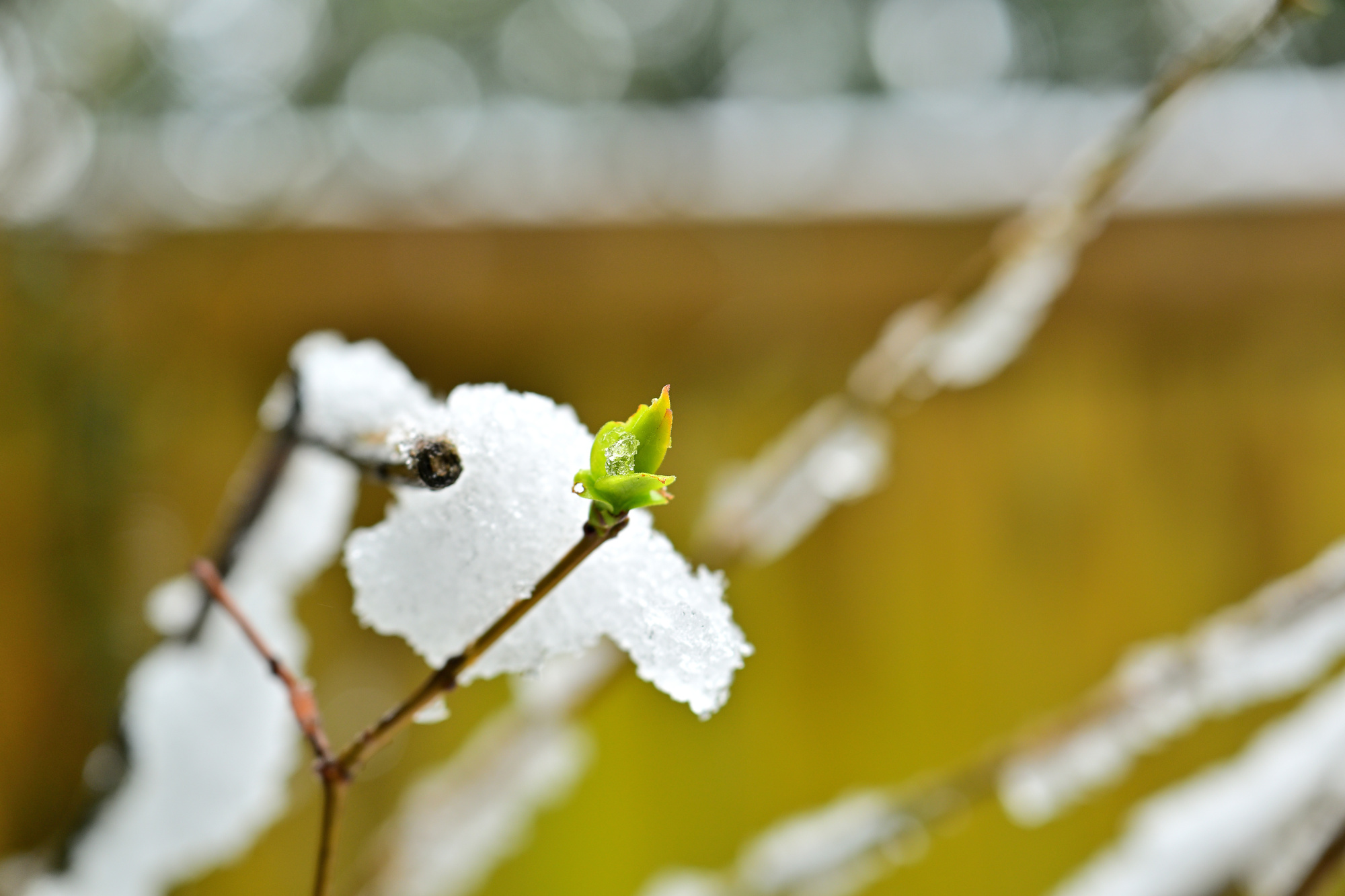
1/100s f/6,3 ISO 100/21° 16-50mm f/2,8 VR f=23mm/34mm
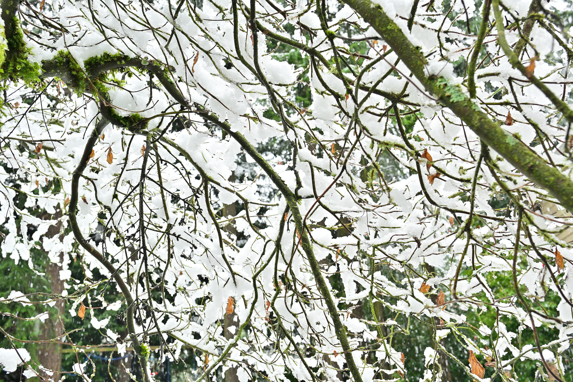
1/160s f/4 ISO 100/21° 16-50mm f/2,8 VR f=29mm/44mm
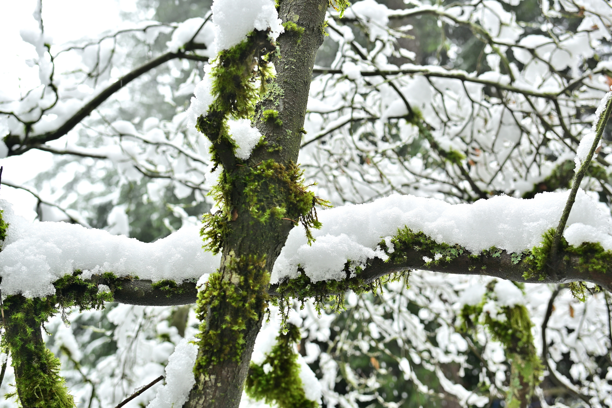
Architektur im Kleinen: Katzentreppe
1/60s f/6,3 ISO 100/21° 16-50mm f/2,8 VR f=20mm/30mm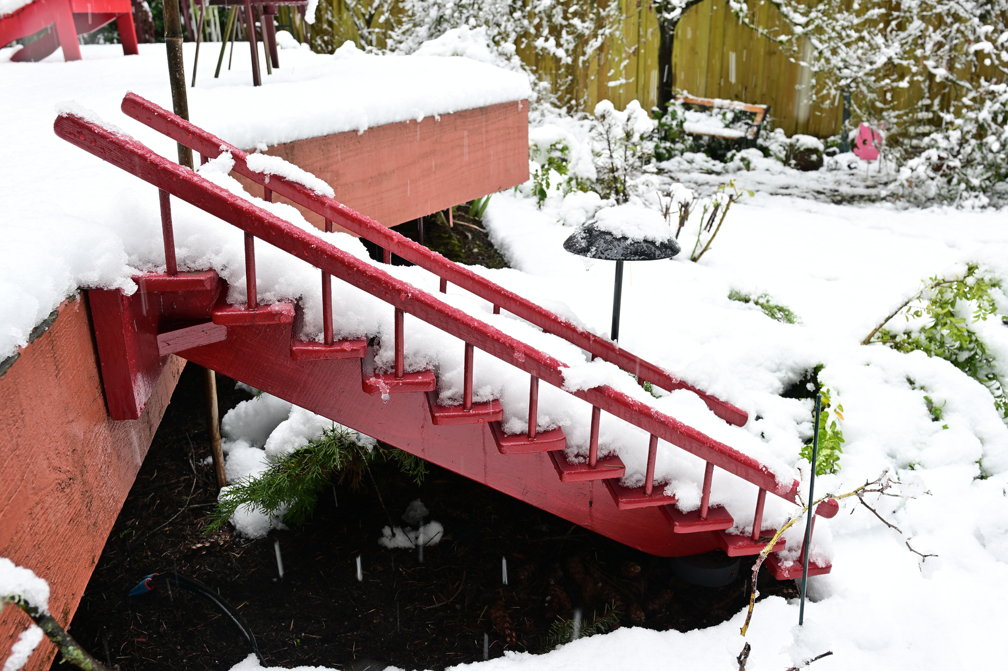
1/40s f/3,2 ISO 100/21° 16-50mm f/2,8 VR f=50mm/75mm
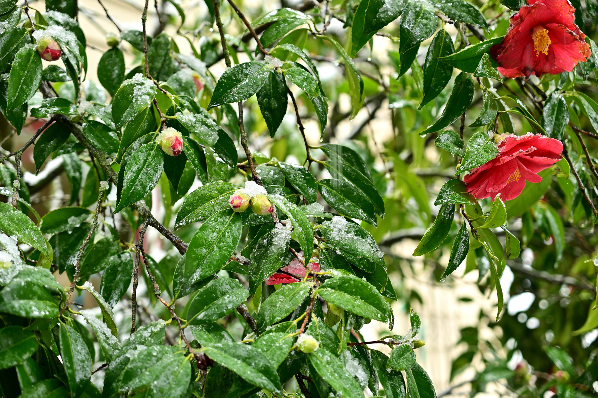
1/160s f/2,8 ISO 100/21° 16-50mm f/2,8 VR f=50mm/75mm
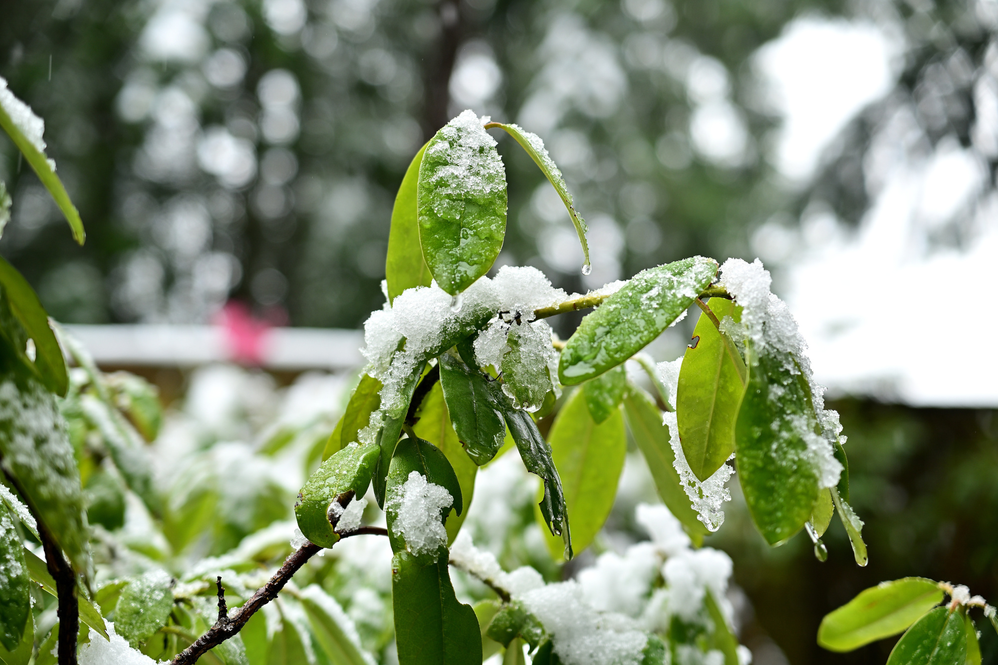
1/400s f/2,8 ISO 100/21° 16-50mm f/2,8 VR f=37mm/55mm
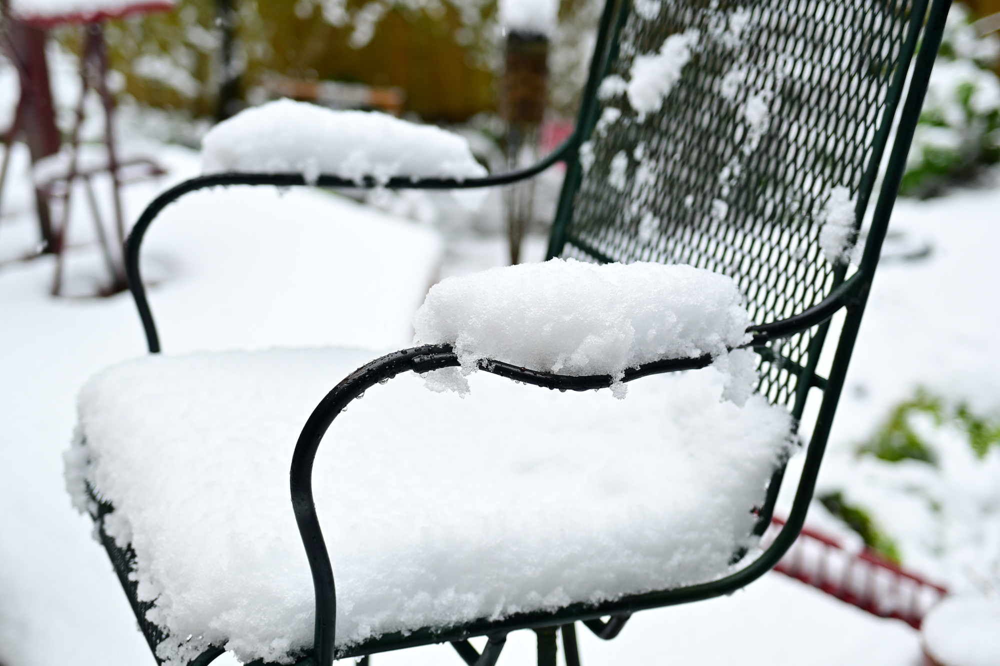
1/160s f/4,5 ISO 100/21° 16-50mm f/2,8 VR f=26mm/39mm
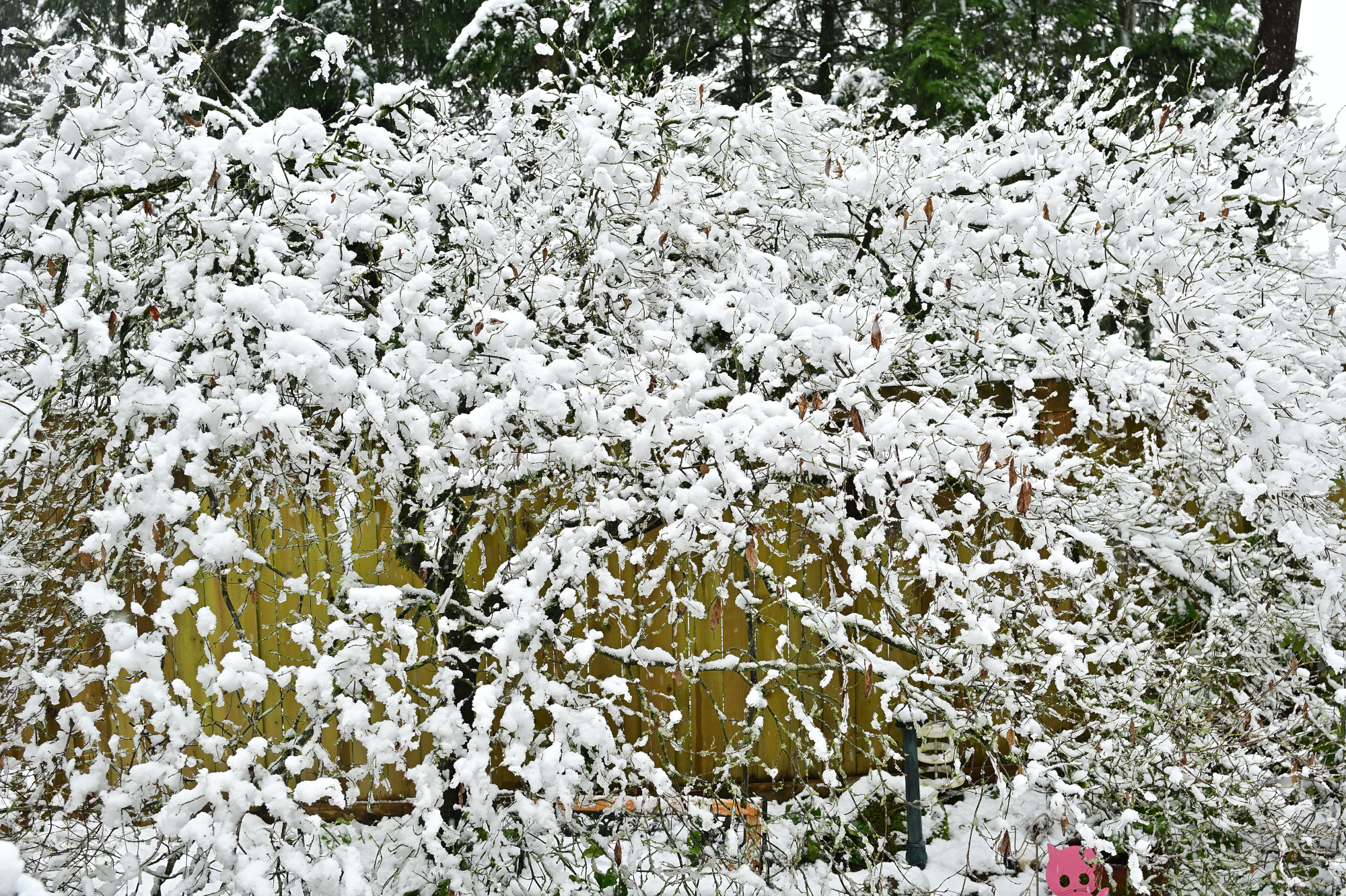
1/60s f/4,5 ISO 100/21° 16-50mm f/2,8 VR f=19mm/29mm
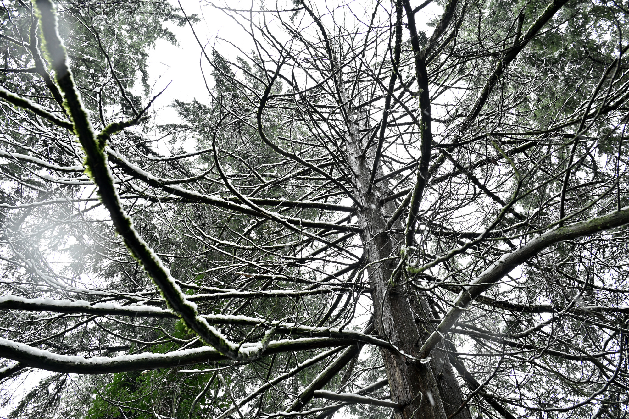
1/60s f/4,5 ISO 100/21° 16-50mm f/2,8 VR f=50mm/75mm
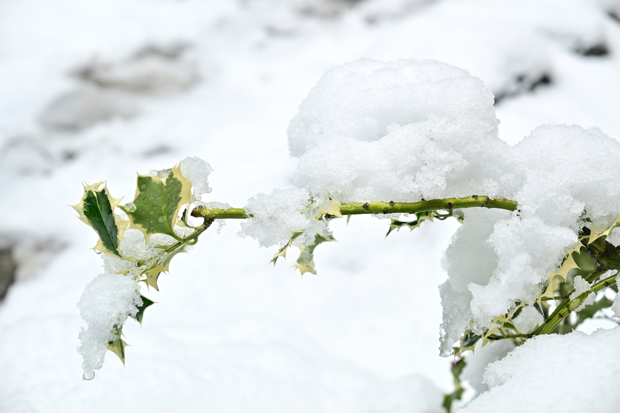
Diese Bilder sind Teil einer neuen Arbeitsweise.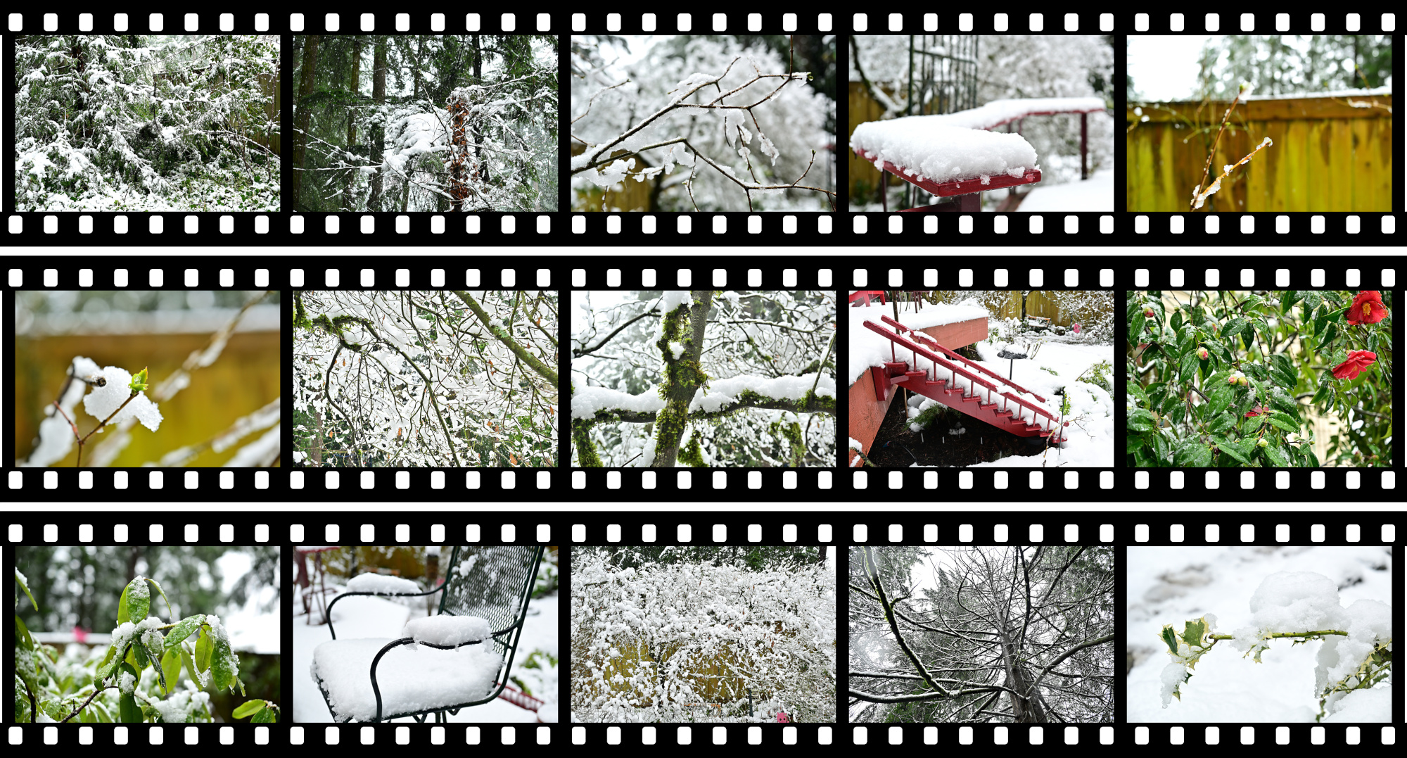
-
Lossless Exposure & Contrast Adjustment in JPEG10
Lossless Tonal Adjustments in JPEG's DCT Domain: Exposure Compensation and Multi-Band Contrast
Most JPEG workflows treat exposure (brightness) and contrast as inherently "lossy": decode pixels, apply curves, then re-encode. That approach works, but it always introduces an additional step of quantization error.
In this github fork of the IJG JPEG-10 code, I added two options to
jpegtranthat operate directly on quantized DCT coefficients:-exposure-comp EV-contrast DC LOW MID HIGH
Both are applied during transcoding, so they combine naturally with existing
jpegtranoperations such as rotation, flipping, cropping, marker copying, and progressive conversion.https://github.com/jurgen178/jpeg10
Download Windows x64 binary: jpegtran.zip
Quick Usage
jpegtran [standard options] [-exposure-comp EV] [-contrast DC LOW MID HIGH] input.jpg output.jpgExamples:
# Brighten by 1 stop
jpegtran -copy all -exposure-comp 1 input.jpg output.jpg

# Darken by 0.5 stops
jpegtran -copy all -exposure-comp -0.5 input.jpg output.jpg

# Contrast (uniform: DC=LOW=MID=HIGH)
jpegtran -copy all -contrast -1   -1   -1   -1   input.jpg out-contrast-u-1.jpg
jpegtran -copy all -contrast -0.5 -0.5 -0.5 -0.5 input.jpg out-contrast-u-0.5.jpg
jpegtran -copy all -contrast  0.5  0.5  0.5  0.5 input.jpg out-contrast-u+0.5.jpg
jpegtran -copy all -contrast  1    1    1    1   input.jpg out-contrast-u+1.jpg

# Contrast (band-specific examples)
jpegtran -copy all -contrast 0 0 0.6 0   input.jpg out-contrast-mid+0.6.jpg
jpegtran -copy all -contrast 0 0 0 0.4   input.jpg out-contrast-high+0.4.jpg
jpegtran -copy all -contrast 0 0.4 0 0   input.jpg out-contrast-low+0.4.jpg

# Combine: rotate 90°, brighten 0.5 EV, and add uniform contrast +0.5
jpegtran -copy all -rot 90 -exposure-comp 0.5 -contrast 0.5 0.5 0.5 0.5 input.jpg output.jpg
Both switches accept fractional values. Practical ranges:
Option Practical range Neutral -exposure-comp EV-3 … +3 0 -contrast DC LOW MID HIGH-2 … +2 0 Integrated into cPicture with live preview:
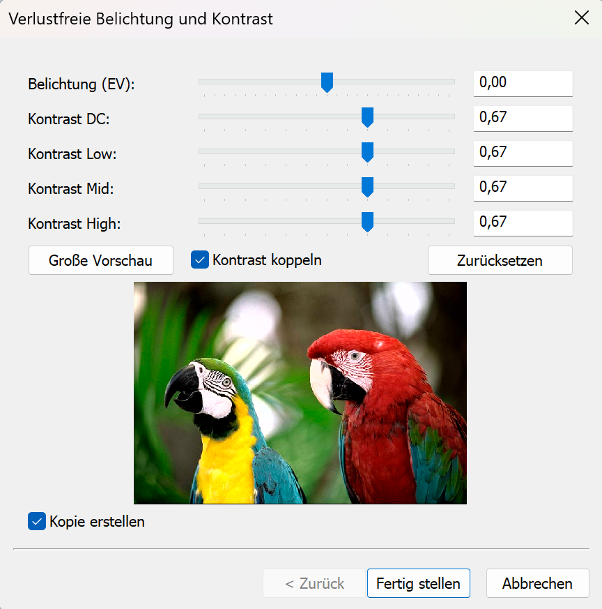
Background: DCT Coefficient Basics
A JPEG image is encoded as a grid of DCT blocks (with 8×8 Elements in size). Each block has one DC coefficient and 63 AC coefficients. But each MCU might have more than one block depending on the color subsampling.
-
DC[0] represents the (level-shifted) average sample value of the block. The relationship to pixel mean is:
$$\mu = \frac{DC_\text{unquant}}{N} + \text{center}$$
where $N$ is the DCT block size of 8 and $\text{center} = 2^{\text{precision}-1}$ (e.g. 128 for 8‑bit).
-
AC[1..N²−1] represent spatial frequency components (texture, edges, contrast).
Both DC and AC are stored quantized: the actual stored integer is $\text{round}(\text{value} / Q_k)$, where $Q_k$ is the quantization step for coefficient $k$.
-exposure-comp EV— Exposure CompensationExposure compensation from -2EV to +2EV:

Concept
A photographic EV step corresponds to doubling (or halving) the amount of light. Applied in linear light:
$$\text{gain} = 2^{EV}$$
Because JPEG samples are gamma-coded (sRGB), pixel values cannot be multiplied directly. Instead:
- Estimate a representative level from the DC blocks.
- Compute the equivalent additive pixel-domain offset by applying the gain in linear light at that reference level.
- Translate the offset into a quantized DC delta.
- Add the delta to every DC coefficient.
Only DC is modified. AC coefficients are not modified, so local contrast and texture are preserved.
Reference Level — Log-Average
A geometric mean (log-average) of all block mean levels is used as the exposure reference:
$$\bar{L} = \exp\!\left(\frac{1}{B}\sum_{i=1}^{B} \ln(L_i + 1)\right) - 1$$
where $L_i$ is the intensity mean of block $i$ (clamped to $[0, \text{MAX}]$) and $B$ is the total number of blocks.
sRGB Linearisation
The gain is applied in linear light:
$$u_\text{ref} = \frac{\bar{L}}{\text{MAX}}$$
$$u_\text{ref,lin} = f_\text{lin}(u_\text{ref})$$
$$u_\text{new,lin} = \min(u_\text{ref,lin} \cdot \text{gain},\; 1.0)$$
$$u_\text{new} = f_\text{sRGB}(u_\text{new,lin})$$
The sRGB transfer functions used:
$$f_\text{lin}(u) = \begin{cases} u / 12.92 & u \le 0.04045 \\ \left(\dfrac{u + 0.055}{1.055}\right)^{2.4} & u > 0.04045 \end{cases}$$
$$f_\text{sRGB}(u) = \begin{cases} 12.92\,u & u \le 0.0031308 \\ 1.055\,u^{1/2.4} - 0.055 & u > 0.0031308 \end{cases}$$
Pixel-Domain Offset → Quantized DC Delta
$$\Delta_\text{samples} = (u_\text{new} - u_\text{ref}) \cdot \text{MAX}$$
Clamped to available headroom/shadow room to limit clipping, then converted to a quantized DC delta:
$$\Delta_{DC} = \text{round}\!\left(\frac{\Delta_\text{samples} \cdot N}{Q_0}\right)$$
where $N$ is the DCT block size and $Q_0$ is the DC quantization step.
Component Policy
Color space Components adjusted YCbCr, BG_YCC, YCCK Luma only (component 0) RGB/BG_RGB + subtract-green transform Green/base only (component 1) CMYK, all others All components For CMYK and YCCK the delta is computed in an inverted intensity domain ($I = \text{MAX} - \text{sample}$) so that +EV brightens and −EV darkens.
-contrast DC LOW MID HIGH— Contrast AdjustmentContrast from -1CV to +1CV:

Concept
This option provides four separate controls (all in stops):
DCcontrols the DC coefficient (block mean)LOW,MID,HIGHcontrol the AC coefficients in frequency order
All controls are interpreted as log2 gains (stops). For a value $x$, the gain is:
$$g(x) = 2^{x}$$
So +1 doubles, -1 halves.
DC
DC is scaled by:
$$g_\mathrm{DC} = 2^{DC}$$
and applied as:
$$DC' = \mathrm{clamp}(\mathrm{round}(g_\mathrm{DC} \cdot DC))$$
AC (low/mid/high weighting)
AC coefficients are processed in zigzag order (the JPEG natural order). Let $z$ be the AC position with $z = 1 \ldots A$, where $A$ is the number of AC coefficients.
Define a normalized position:
$$t = \begin{cases} \dfrac{z-1}{A-1} & A > 1 \\ 0 & A = 1 \end{cases}$$
Triangular weights:
- low weight fades out from low frequencies
$$w_\mathrm{low} = \max(0, 1 - 2t)$$
- mid weight peaks in the middle
$$w_\mathrm{mid} = 1 - |2t - 1|$$
- high weight fades in toward high frequencies
$$w_\mathrm{high} = \max(0, 2t - 1)$$
Per-coefficient exponent and gain:
$$v(z) = LOW\cdot w_\mathrm{low} + MID\cdot w_\mathrm{mid} + HIGH\cdot w_\mathrm{high}$$
$$g(z) = 2^{v(z)}$$
Applied to each AC coefficient:
$$AC'[z] = \mathrm{clamp}(\mathrm{round}(g(z)\cdot AC[z]))$$
If
DC = LOW = MID = HIGH = X, then all coefficients are scaled by the same gain $2^X$ (uniform contrast adjustment).Component Policy
Same as
-exposure-comp:- YCbCr/BG_YCC/YCCK: luma only
- RGB subtract-green: base/green only
- otherwise: all components
Ordering and Composition
Both
-exposure-compand-contrastare applied as a post step after any geometric transform (-rot,-flip,-crop, …). The tonal operations work on the final output coefficient arrays, so the order of switches on the command line does not matter.
Implementation notes
- Core implementation:
transupp.c:do_exposure_comp()anddo_contrast()transupp.h: adds new fields tojpeg_transform_info
- CLI parsing:
jpegtran.c
- Feature flags and parameters are stored in
jpeg_transform_infointransupp.h
Summary
-exposure-comp EVshifts brightness by changing only DC coefficients, with EV evaluated in linear light (sRGB transfer) at a log-average reference.-contrast DC LOW MID HIGHscales DC and AC coefficients, with AC gains varying smoothly over frequency order using low/mid/high controls.- Both run in the DCT domain and integrate naturally into the lossless-transformation workflow of
jpegtran.
Example pictures
-
Chagall Fenster der Stephanskirche in Mainz
Chagall-Fenster im Chor
Die Fenster der Stephanskirche wurden von Marc Chagall gestaltet und prägen den gesamten Raum. Das tiefe Blau und die warmen Farbtöne fangen das Licht auf eine Weise ein, die sofort eine besondere Ruhe entstehen lässt. Beim Betreten der Kirche verändert sich die Wahrnehmung fast unmerklich, doch sehr deutlich. Farbe, Licht und Stille verbinden sich zu einem Moment, der lange nachwirkt.
Chagall begann in der zweiten Hälfte der 1970er Jahre damit, für die Stephanskirche Fenster zu entwerfen, damals bereits fast neunzig Jahre alt. Das erste Fenster wurde 1978 eingebaut und war ursprünglich als einzelnes Werk gedacht. Doch er arbeitete weiter. Bis zu seinem Tod 1985 schuf Chagall insgesamt neun Fenster für den vorderen Teil der Kirche. Chagall entwarf die Glasgemälde und führte auch die Schwarzlotmalerei eigenhändig aus. Seine Arbeit verstand er als Zeichen der jüdisch-deutschen Aussöhnung. Nach seinem Tod wurde die Arbeit an den weiteren Fenstern in St. Stephan von Charles Marq fortgesetzt.
Das tiefe Blau, das seine Arbeiten auszeichnet, verändert den ganzen Raum. Das Licht wird weicher, die Farben wirken fast schwebend, und die Kirche bekommt eine Ruhe, die man sofort spürt.
360°-Ansicht aller Fenster, 1/40s f/2 ISO 640/29°
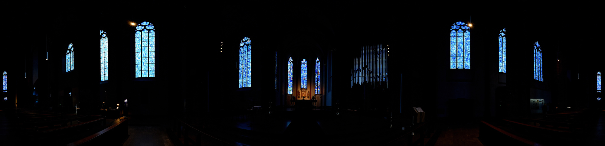
1/50s f/3,5 ISO 800/30° 16-50mm f/2,8 VR f=32mm/48mm
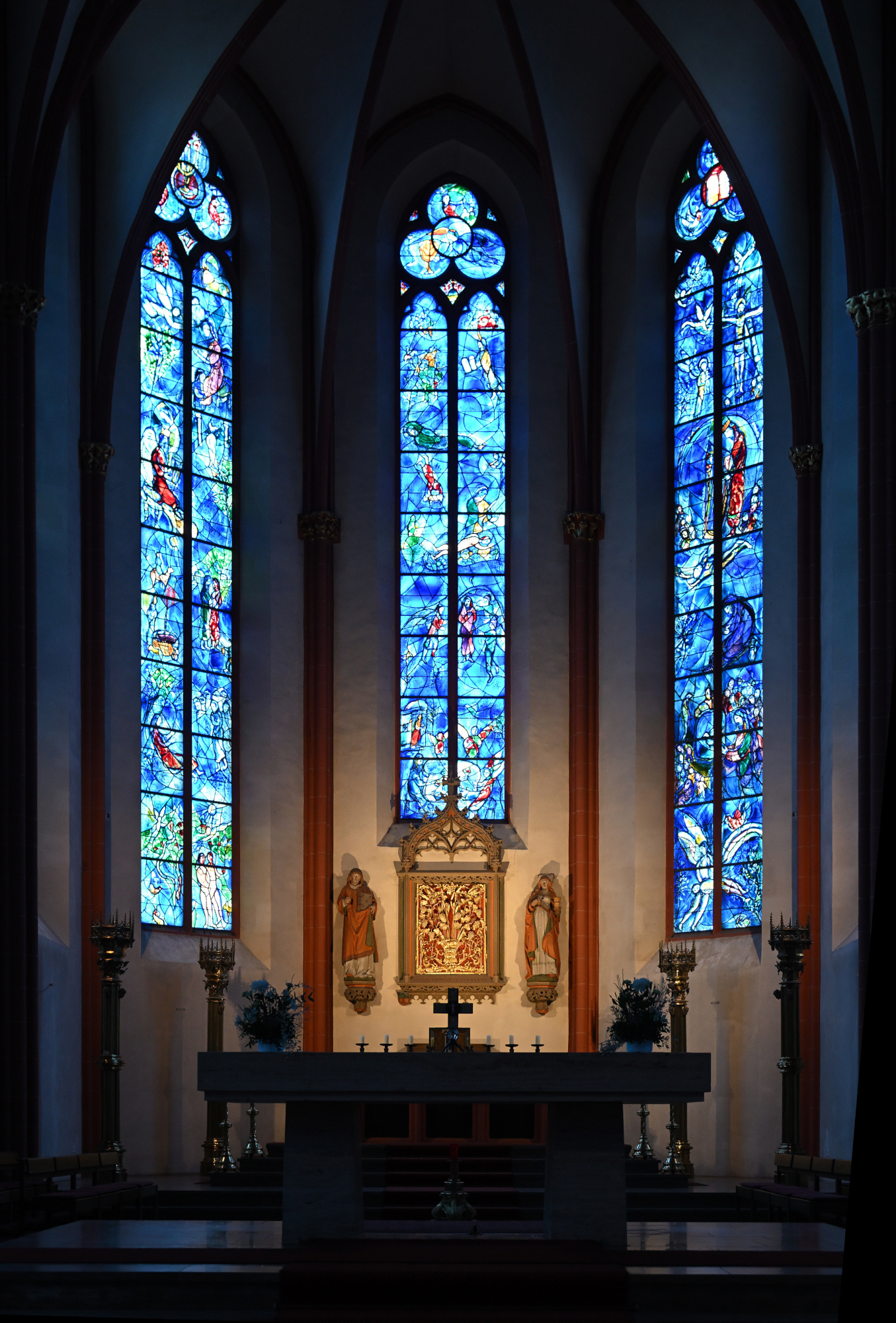
1/25s f/4 ISO 400/27° 16-50mm f/2,8 VR f=22mm/33mm
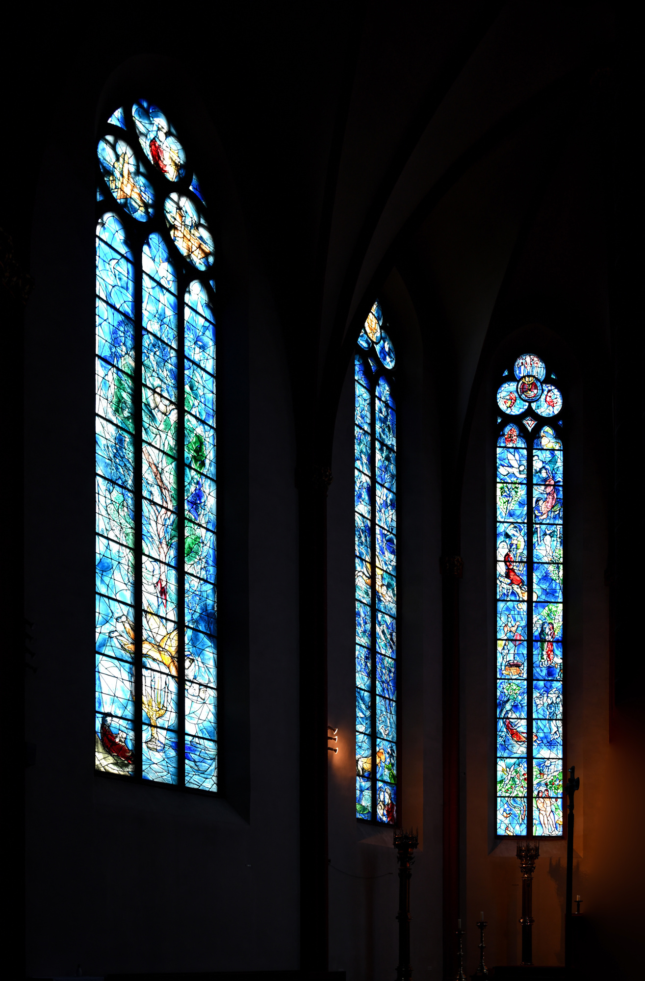
1/20s f/2,8 ISO 250/25° 16-50mm f/2,8 VR f=38mm/57mm
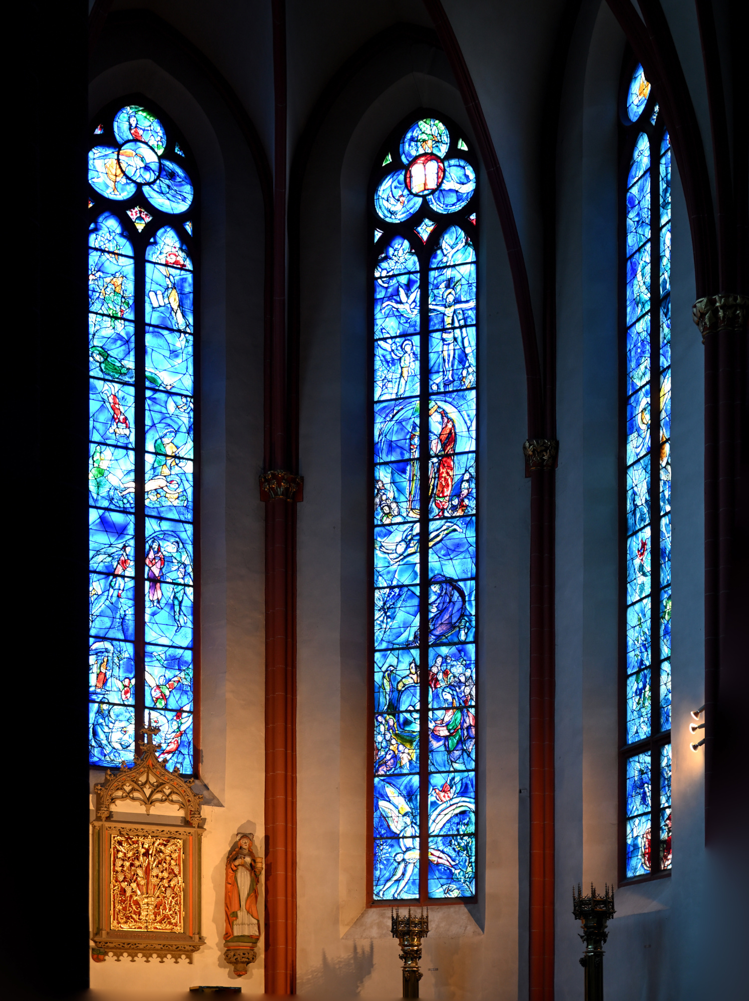
1/30s f/2,8 ISO 250/25° 16-50mm f/2,8 VR f=31mm/46mm
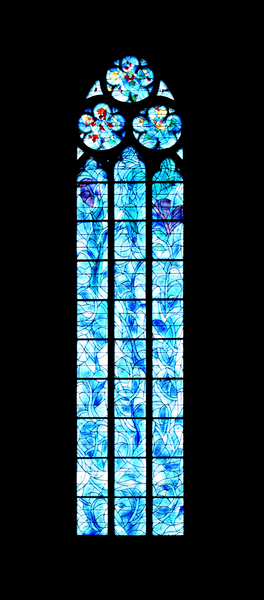
1/30s f/4,5 ISO 400/27° f=13mm
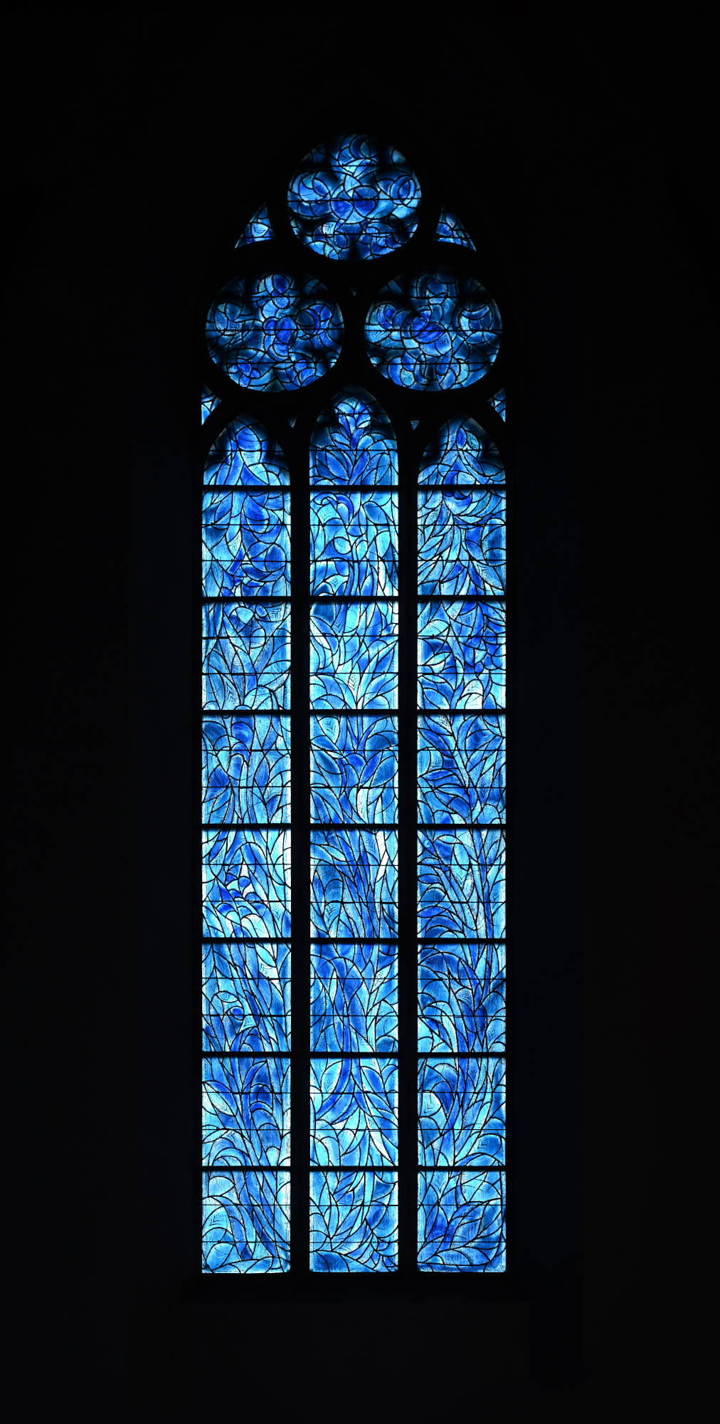
1/25s f/4 ISO 250/25° 16-50mm f/2,8 VR f=30mm/45mm
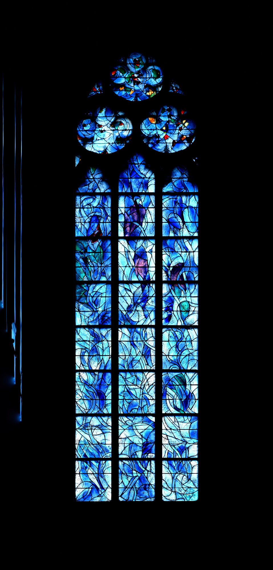
1/13s f/3,5 ISO 400/27° 16-50mm f/2,8 VR f=41mm/61mm
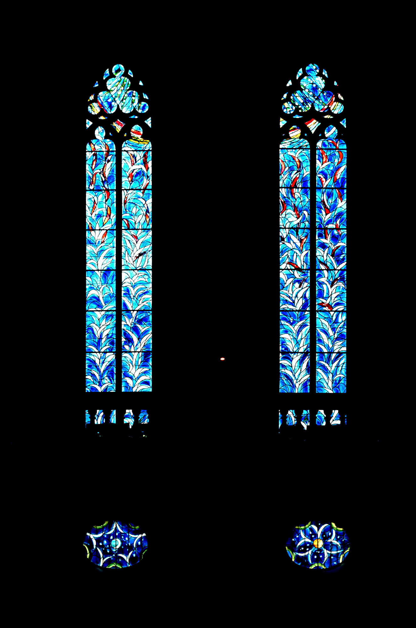
1/40s f/3,2 ISO 800/30° 16-50mm f/2,8 VR f=50mm/75mm
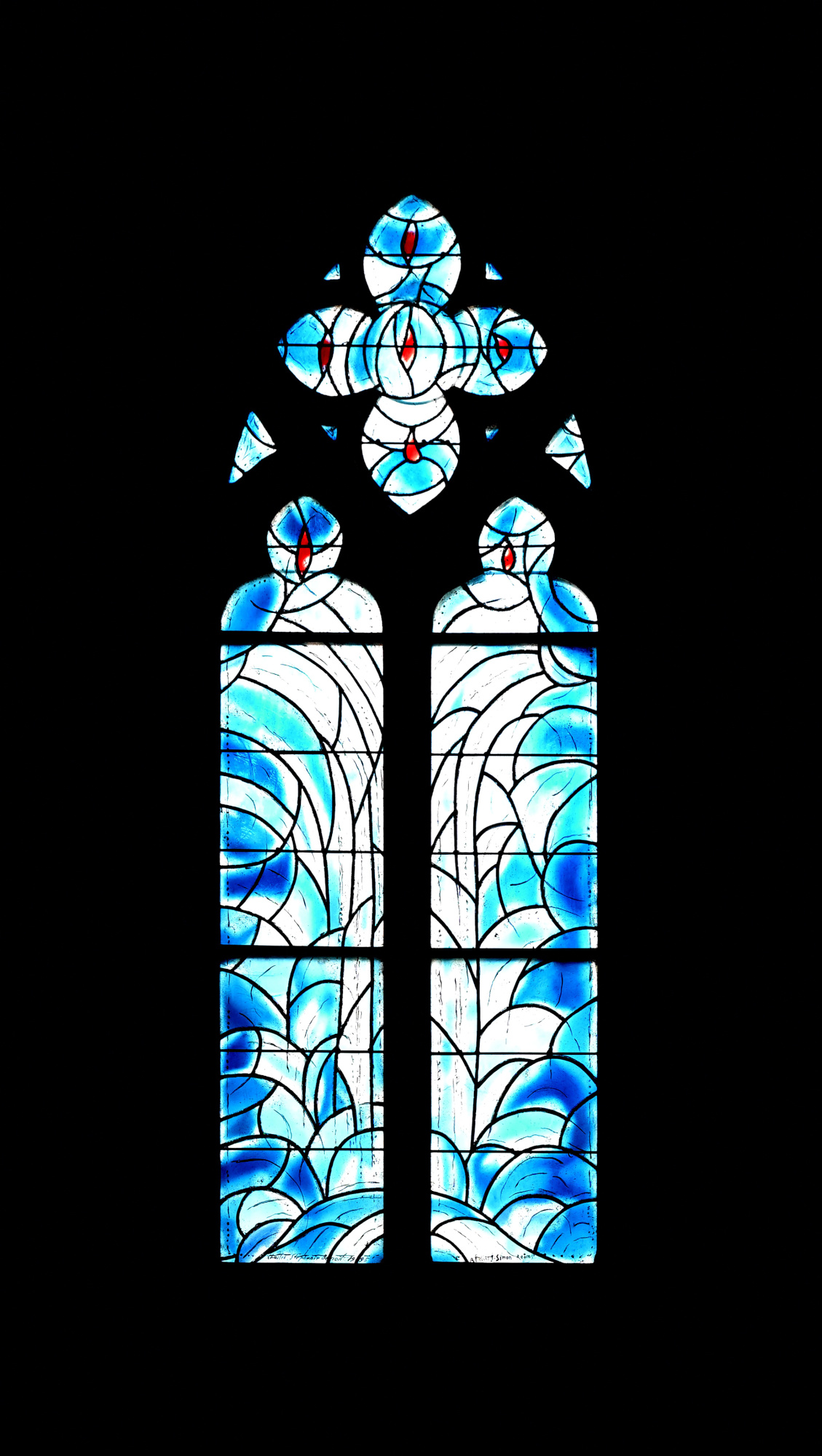
1/50s f/3,5 ISO 800/30° 16-50mm f/2,8 VR f=50mm/75mm
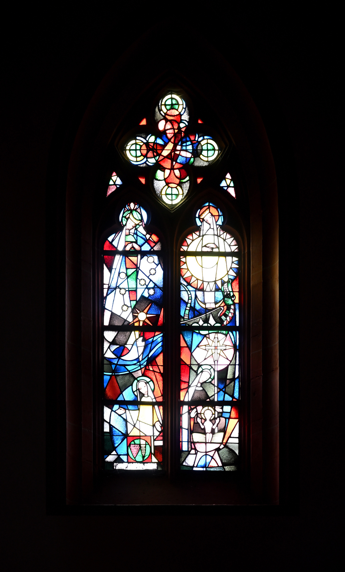
Interaktives Panorama Chagall Fenster der Stephanskirche 1
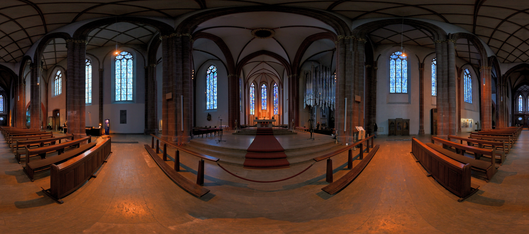
1/50s f/2 ISO 200/24° f=7,5mm

Interaktives Panorama Chagall Fenster der Stephanskirche 2
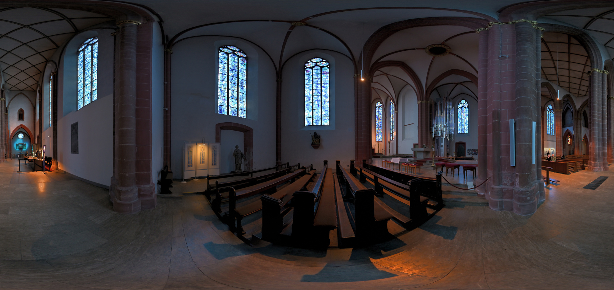
1/50s f/2 ISO 250/25° f=7,5mm

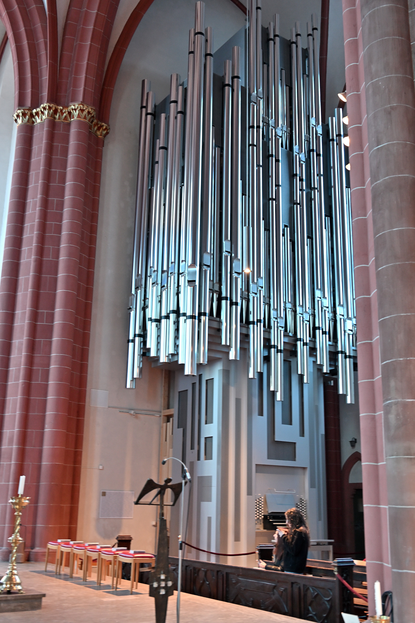
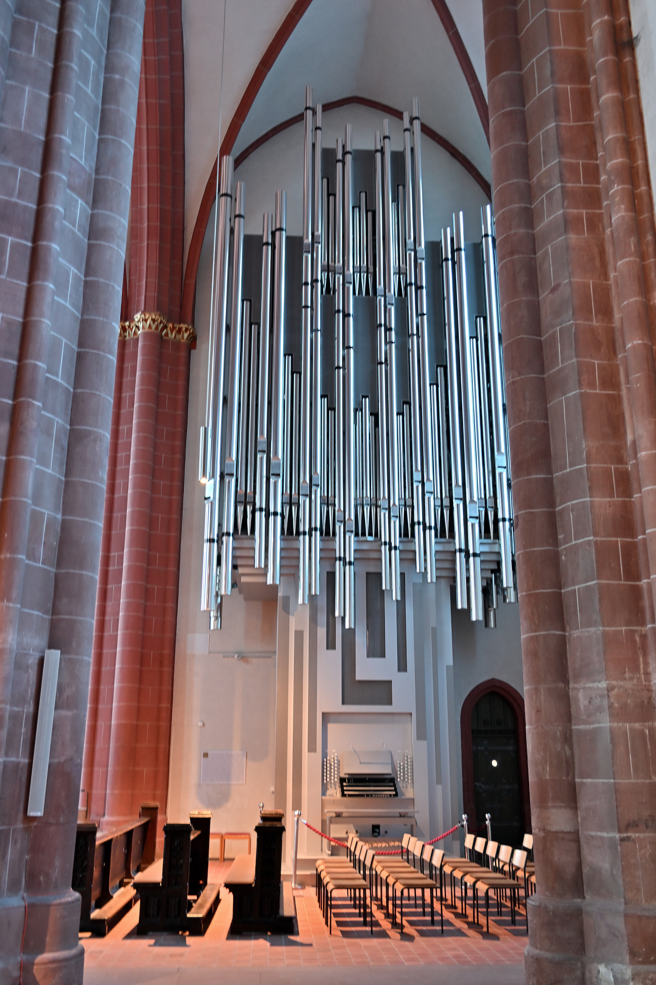
Klais-Orgel im St Stephan, Klang trifft Licht
Die heutige Orgel der Stephanskirche wurde von der Werkstatt Klais aus Bonn gebaut und im Jahr 2013 eingeweiht. Sie entstand nach einem Wettbewerb, bei dem der Entwurf von Klais überzeugte, weil er sich bewusst an der Architektur und am Licht der Kirche orientiert. Die metallischen Flächen der Orgel nehmen die Farben der Chagall Fenster auf und spiegeln sie im Raum wider.
Das Instrument besitzt drei Manuale und Pedal sowie 47 Register und wurde so konzipiert, dass es den weiten Kirchenraum mühelos füllt. Die schlanke Bauweise lässt die Orgel fast wie eine Skulptur wirken, die sich nach oben öffnet und den Raum nicht dominiert, sondern begleitet.
Hier wurde eine längere Belichtungszeit mit niedrigem ISO verwendet, aber die Bildstabilisierung konnte das nicht ganz ausgleichen.
0,3s f/3,5 ISO 400/27° 16-50mm f/2,8 VR f=24mm/36mm
0,4s f/2,8 ISO 250/25° 16-50mm f/2,8 VR f=20mm/30mm
Innenraum der Stephanskirche
1/5s f/2,8 ISO 800/30° 16-50mm f/2,8 VR f=16mm/24mm
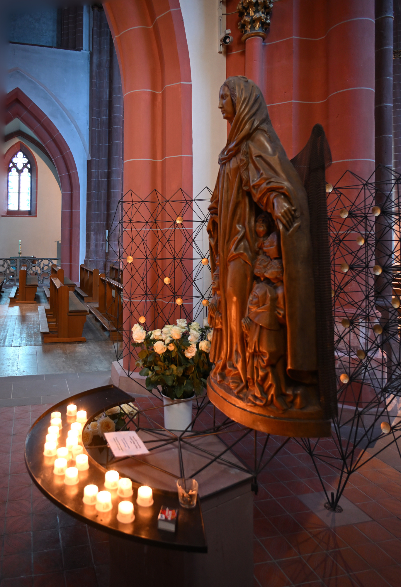
1/30s f/2,8 ISO 800/30° 16-50mm f/2,8 VR f=50mm/75mm
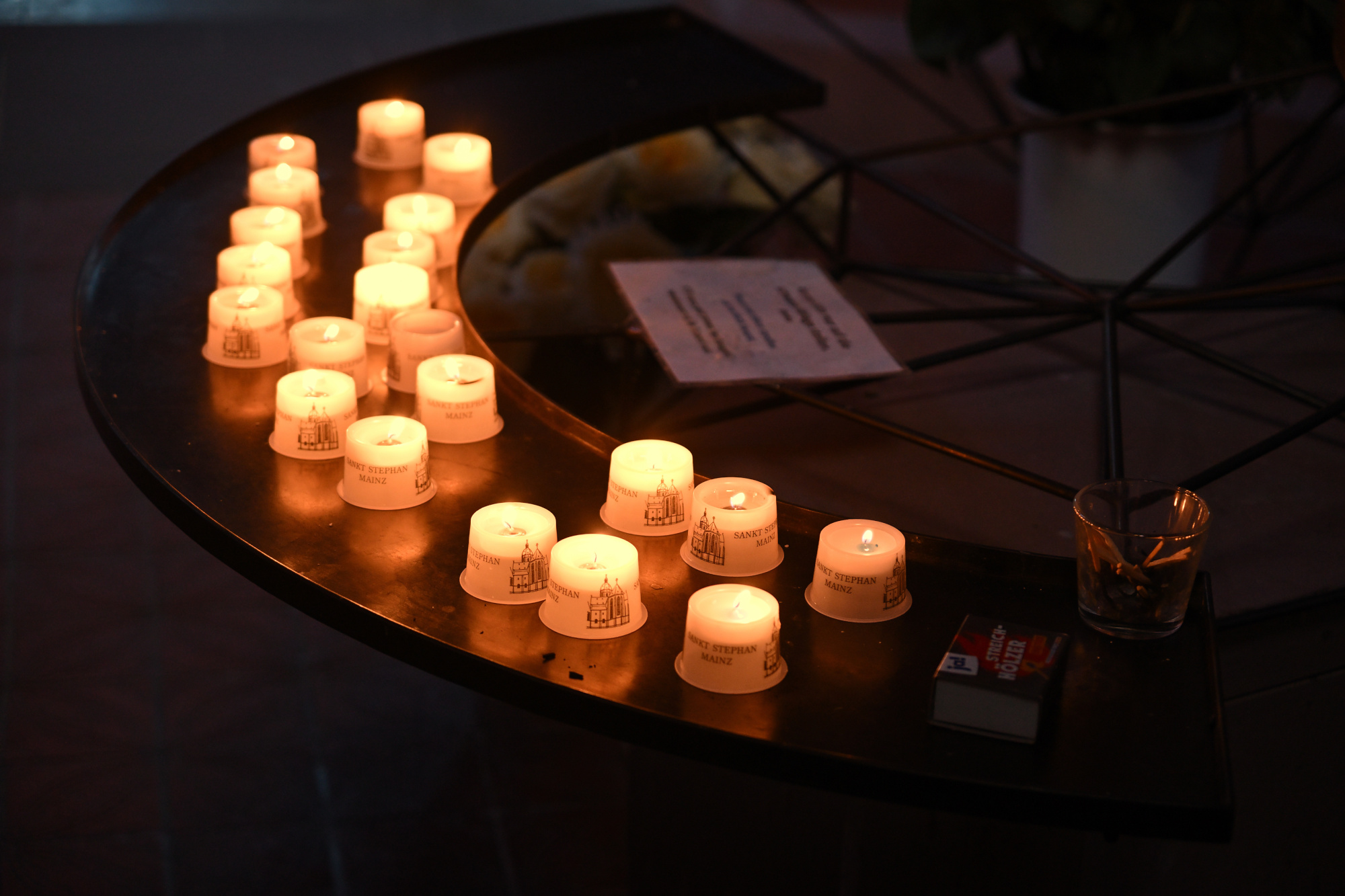
0,3s f/3,5 ISO 1000/31° 16-50mm f/2,8 VR f=26mm/39mm
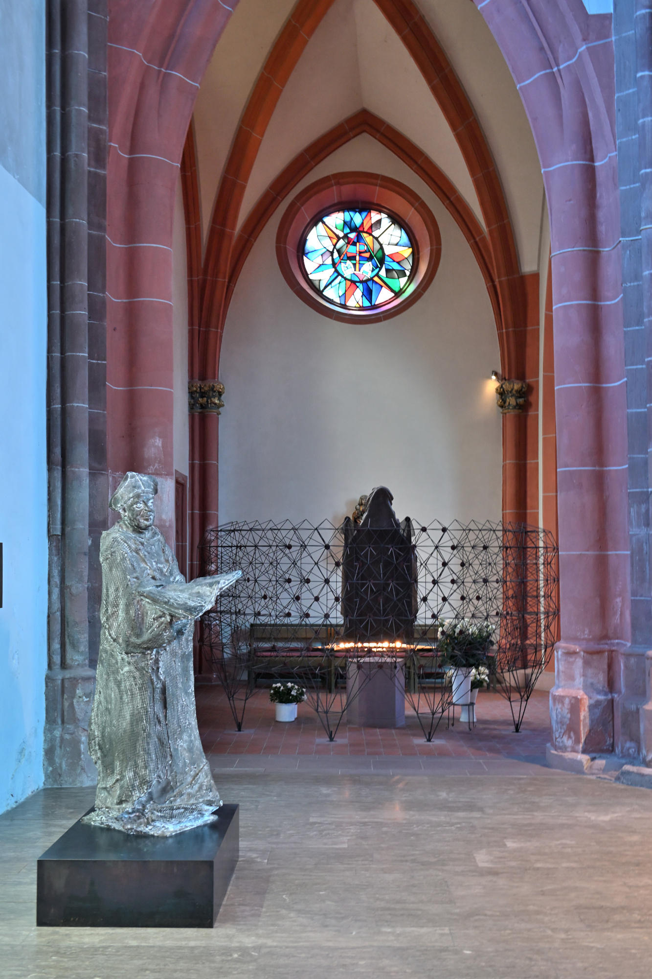
1/25s f/2,8 ISO 800/30° 16-50mm f/2,8 VR f=16mm/24mm
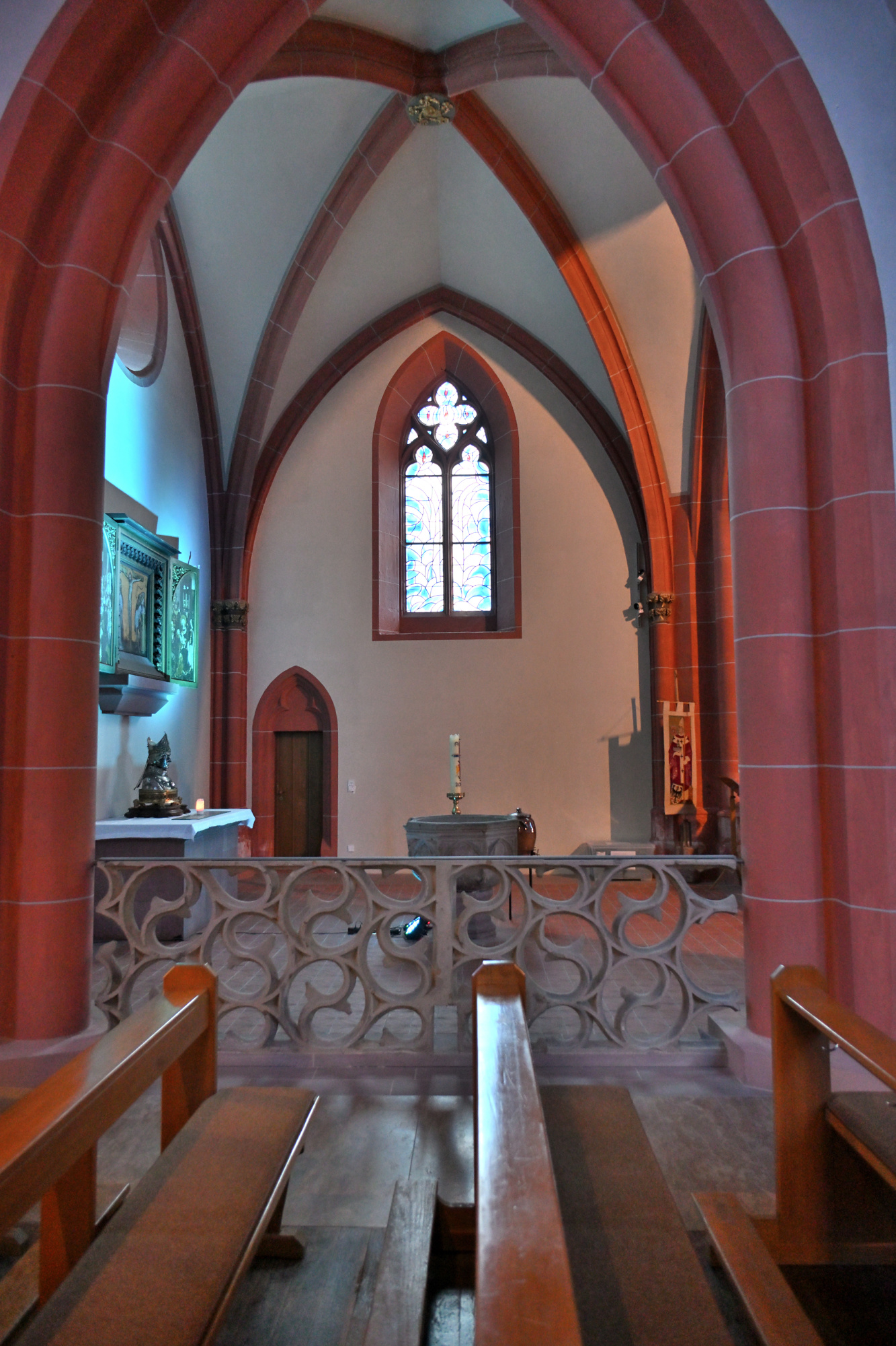
1/25s f/2,8 ISO 800/30° 16-50mm f/2,8 VR f=16mm/24mm
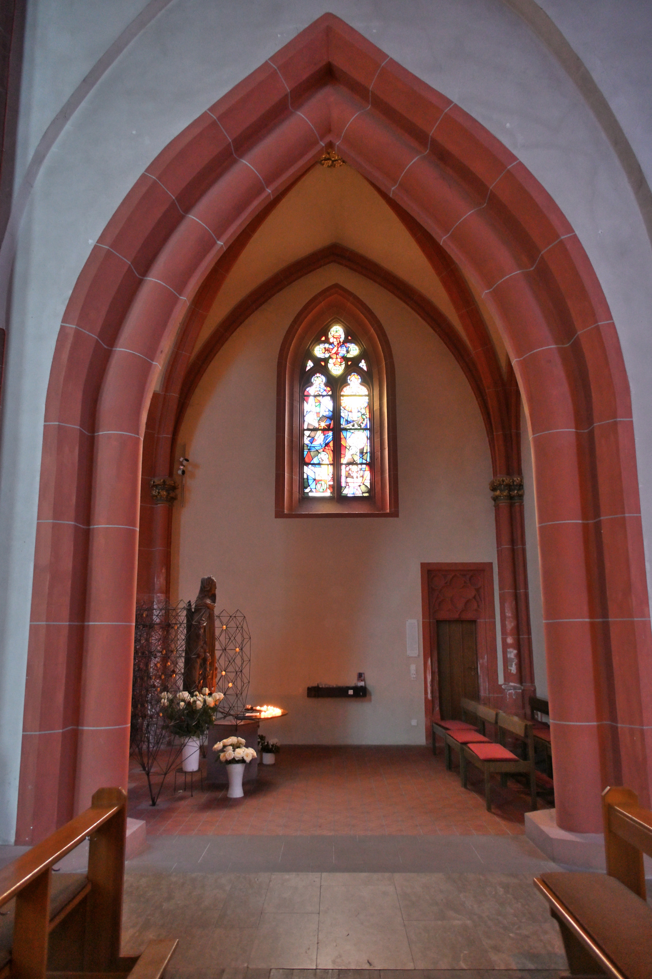
1/50s f/5,6 ISO 640/29° f=7,5mm
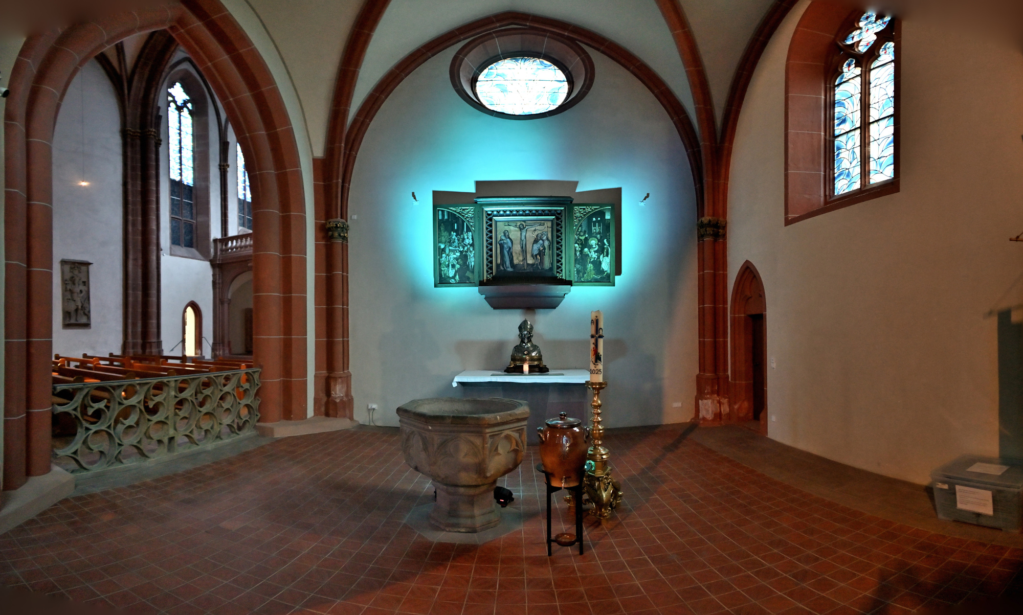
1/8s f/3,5 ISO 1000/31° 16-50mm f/2,8 VR f=28mm/42mm
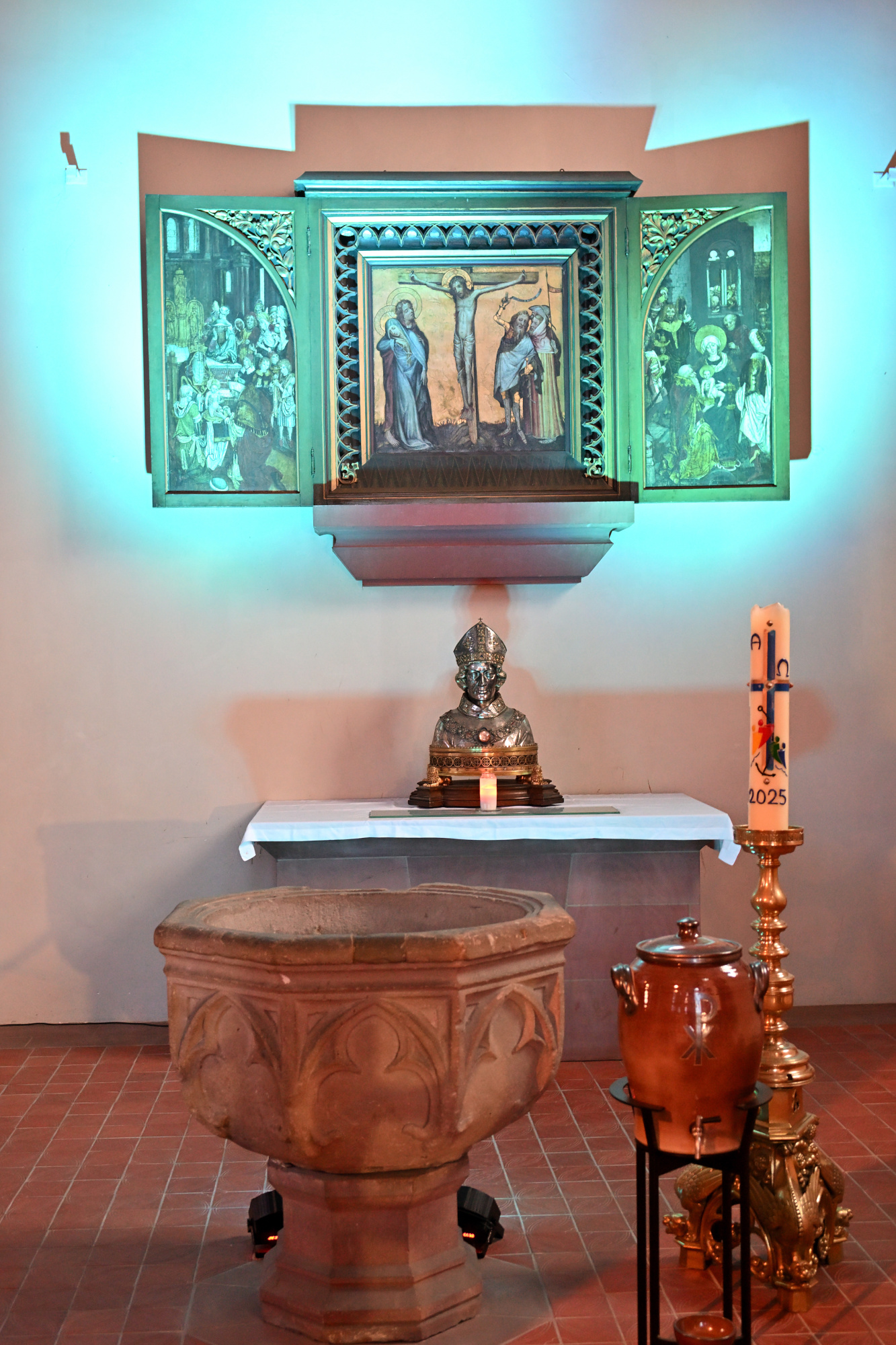
1/13s f/3,5 ISO 1000/31° 16-50mm f/2,8 VR f=16mm/24mm
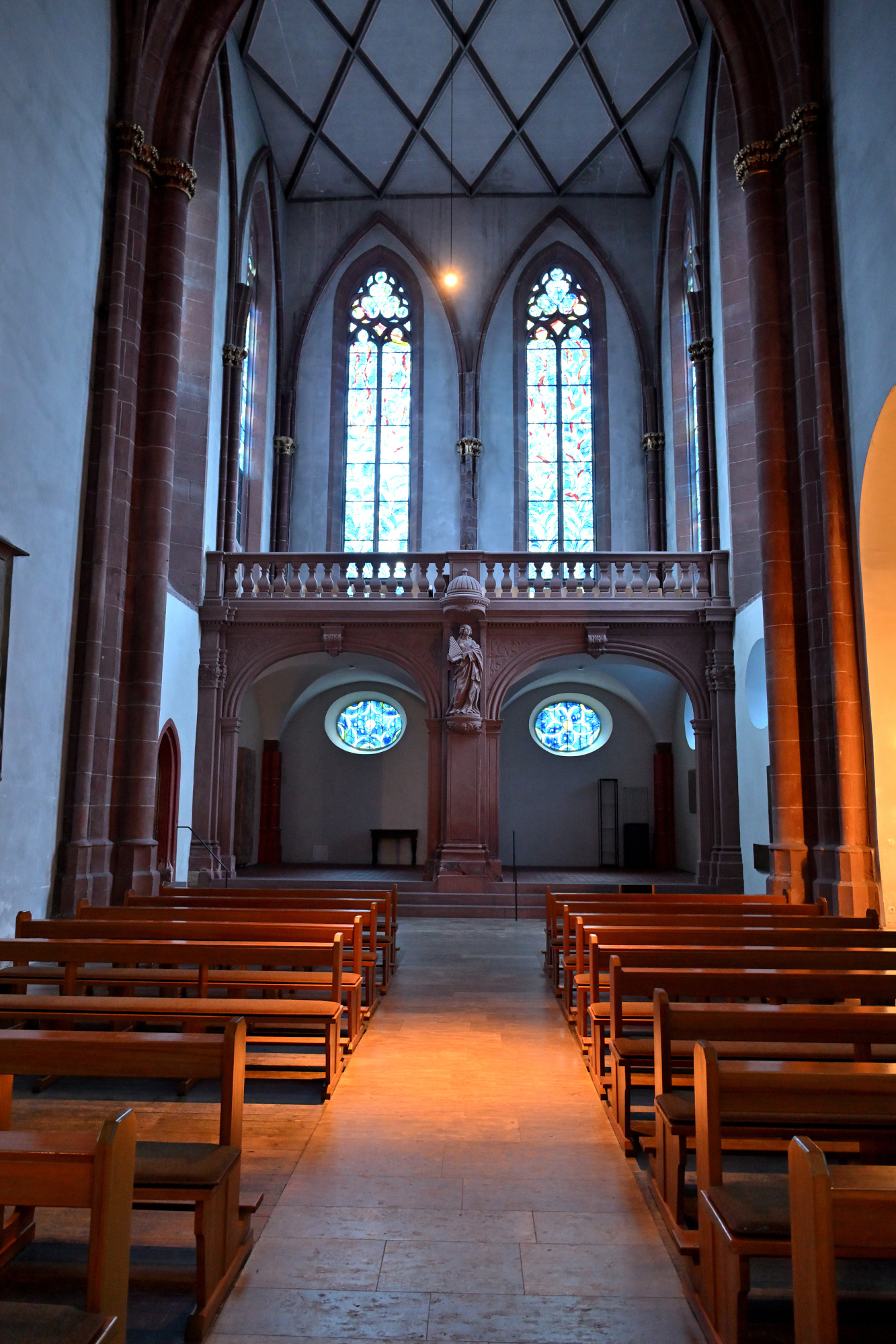
1/15s f/3,5 ISO 1000/31° 16-50mm f/2,8 VR f=16mm/24mm
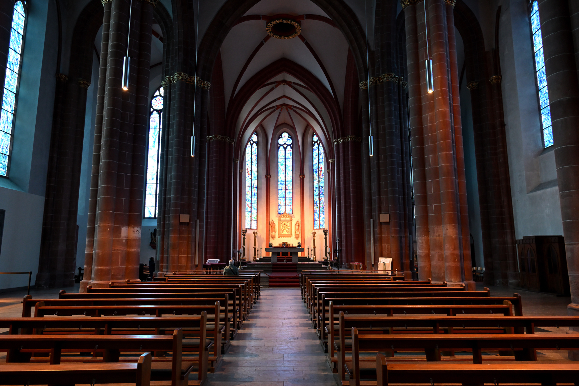
1/5s f/3,5 ISO 400/27° 16-50mm f/2,8 VR f=16mm/24mm
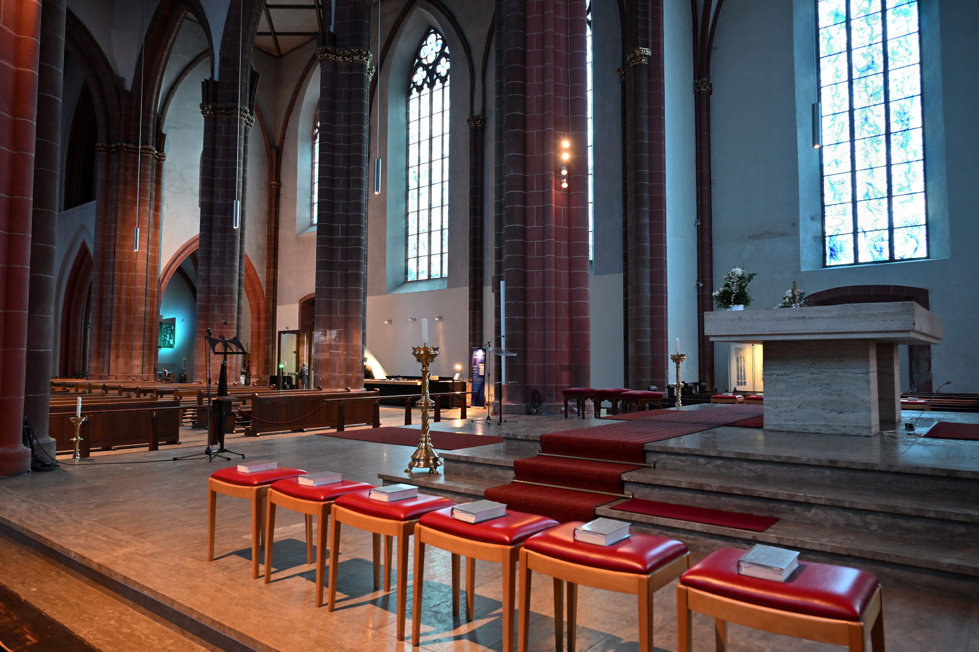
1/25s f/4 ISO 1000/31° 16-50mm f/2,8 VR f=16mm/24mm
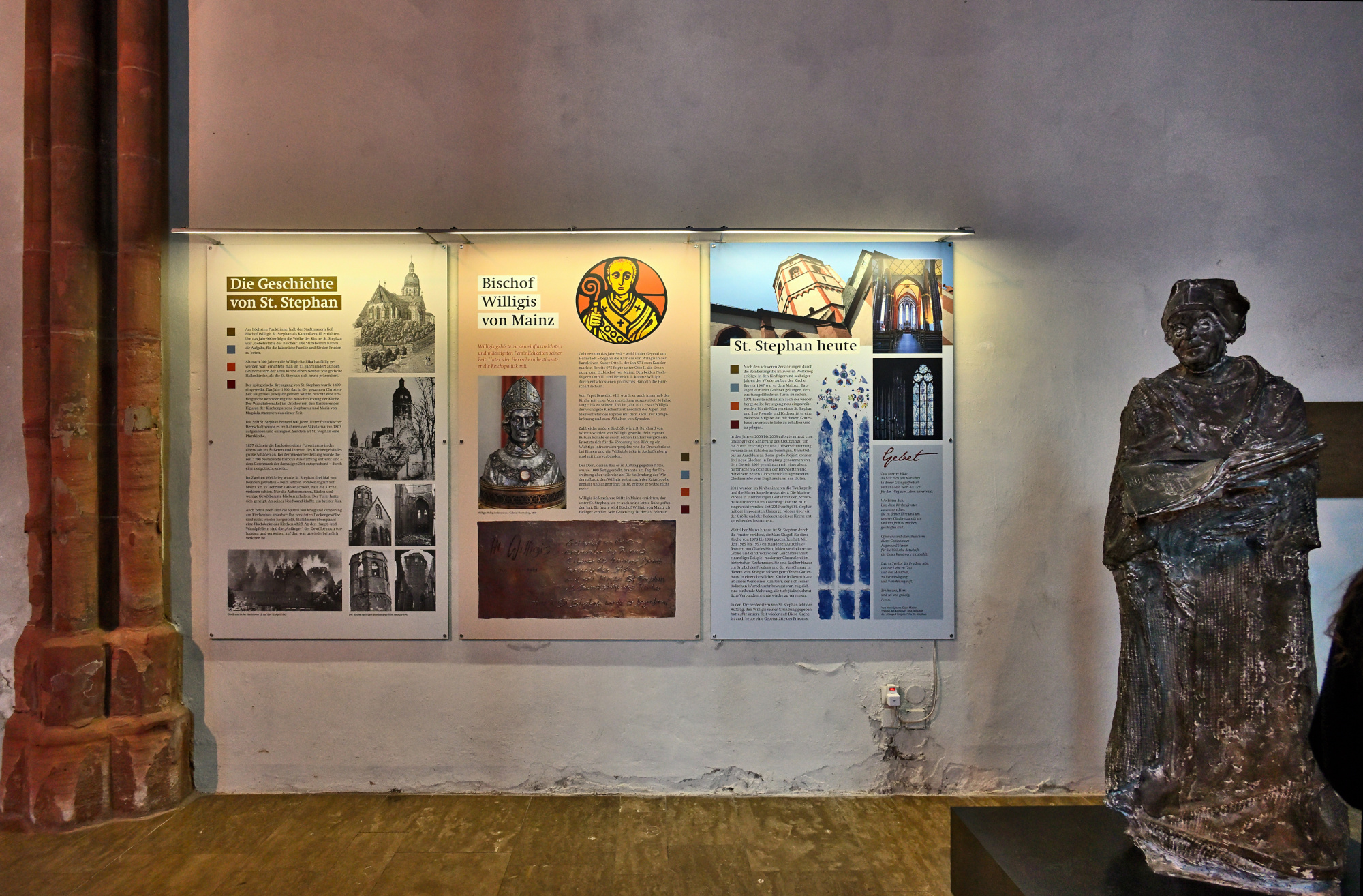
Kreuzgang der Stephanskirche
Der Kreuzgang der Stephanskirche gehört zu den spätgotischen Anlagen der Stadt und wurde im Jahr 1499 vollendet. Er entstand rund eine Generation nach dem Bau der Kirche und wurde von den Stiftsherren in Auftrag gegeben, die damit einen geschützten, ruhigen Bereich an der Südseite der Kirche schufen.
Die Anlage zeigt bis heute viele Spuren ihrer langen Geschichte. An den Wänden stehen zahlreiche Grabplatten, von denen die älteste aus dem Jahr 1048 stammt. Sie wurden im 19. Jahrhundert aus der Kirche hierher gebracht, um sie besser zu erhalten.
Auch der Kapitelsaal gehört zu diesem Ensemble. Seine Mittelsäule wurde bereits um das Jahr 780 geschaffen und später als Abgabe an das Stift übergeben, bevor sie hier ihren Platz fand.
Der Kreuzgang wurde im Laufe der Jahrhunderte mehrfach beschädigt, unter anderem durch die Explosion eines Pulverturms im Jahr 1857 und später im Zweiten Weltkrieg. Zwischen 1968 und 1971 wurde er sorgfältig wiederhergestellt.
Heute wirkt der Innenhof trotz seiner Geschichte leicht und offen. Wer dort entlanggeht, spürt die Ruhe des Ortes und die vielen Schichten der Vergangenheit, die sich in den Mauern gesammelt haben.
1/40s f/5,6 ISO 100/21° f=7,5mm
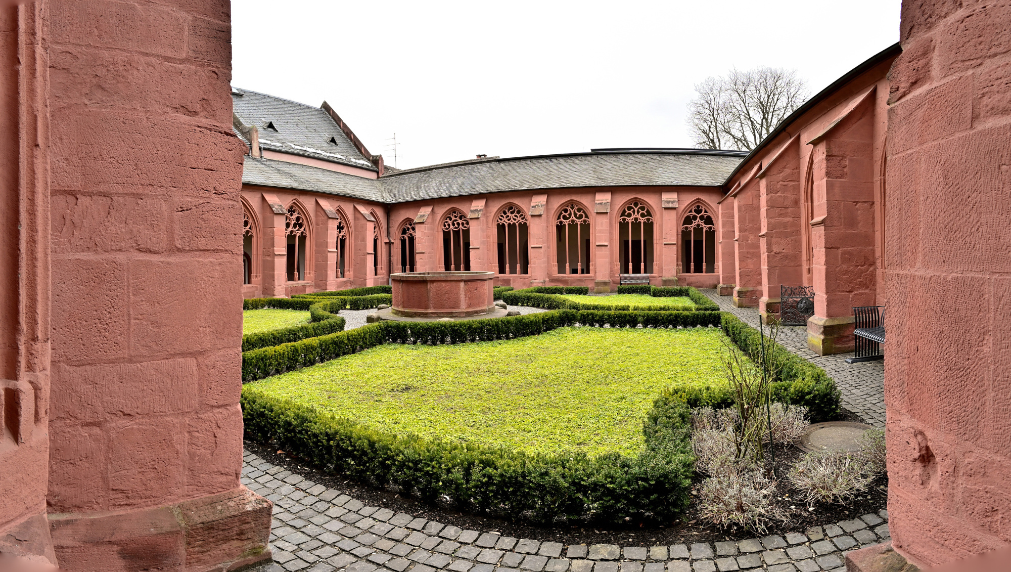
1/40s f/5,6 ISO 100/21° f=7,5mm
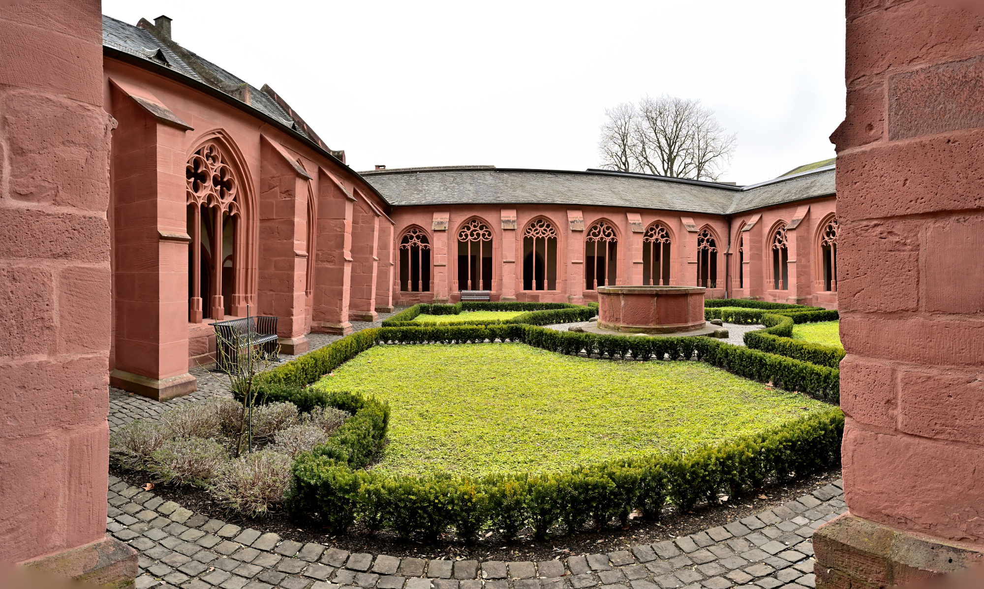
1/60s f/5,6 ISO 100/21° f=7,5mm
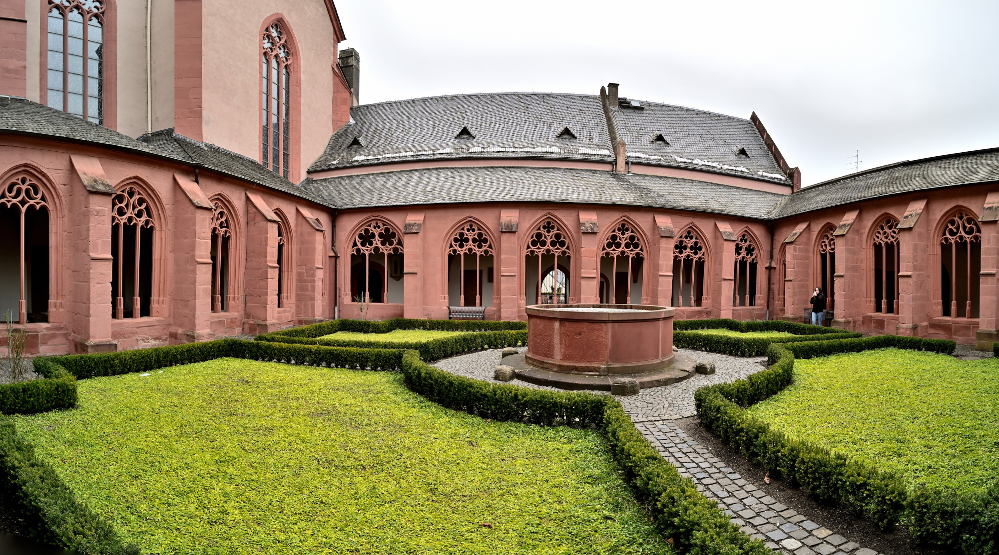
1/50s f/5,6 ISO 100/21° f=7,5mm
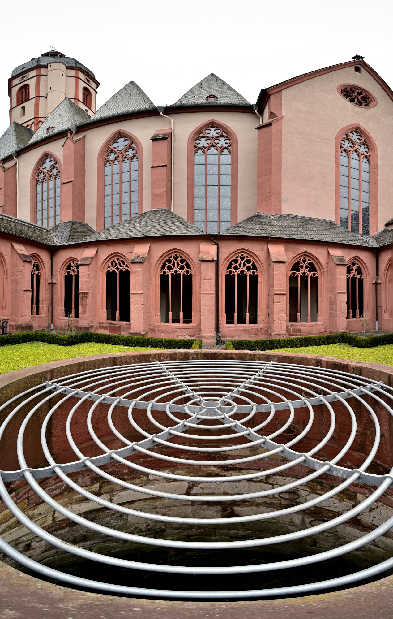
Kreuzgang-Ecken
1/40s f/5,6 ISO 640/29° f=7,5mm
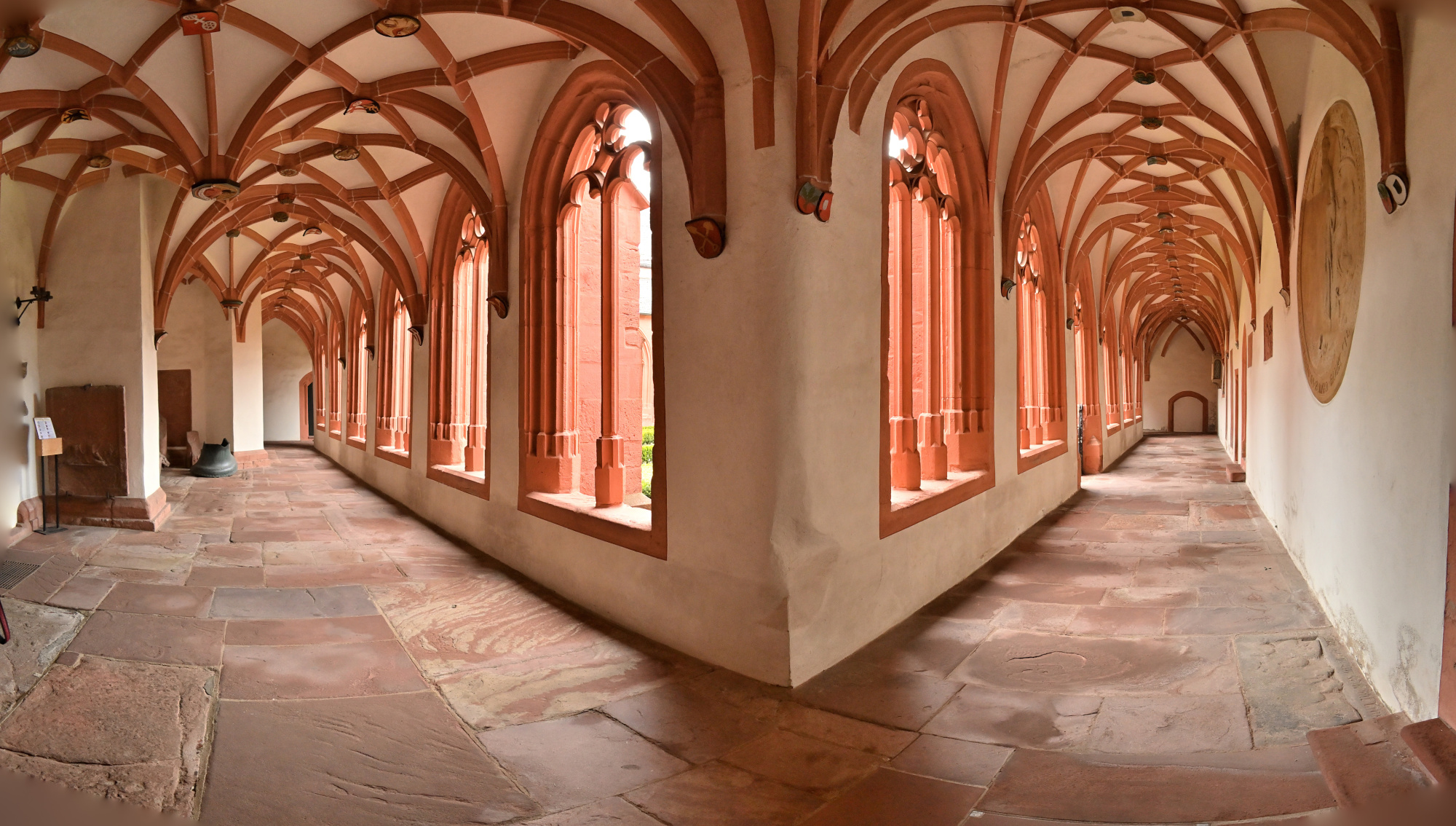
1/40s f/5,6 ISO 640/29° f=7,5mm
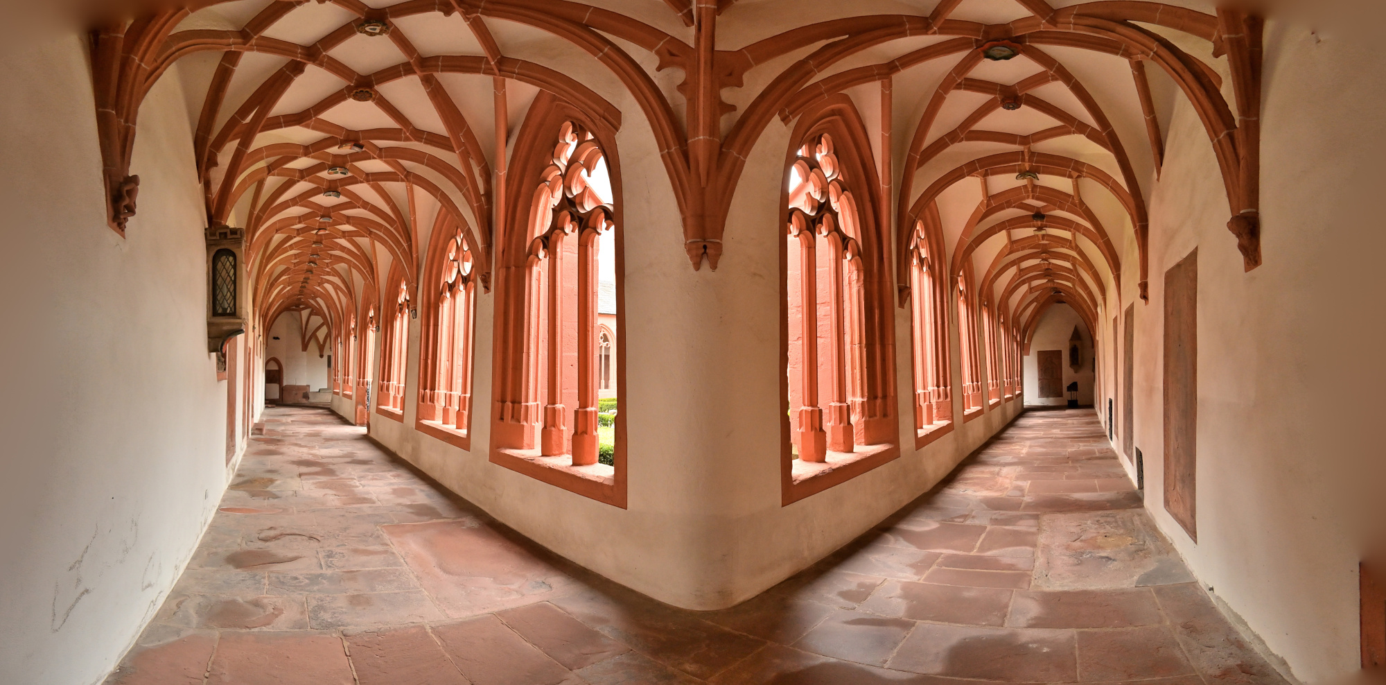
1/40s f/5,6 ISO 640/29° f=7,5mm
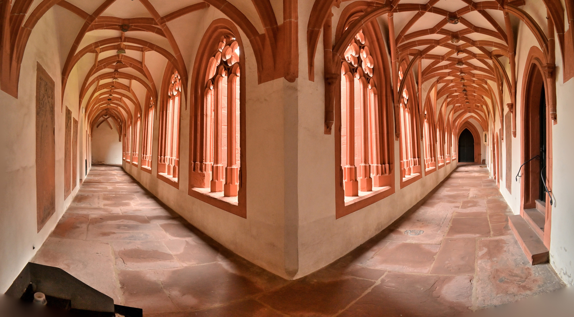
1/40s f/5,6 ISO 640/29° f=7,5mm
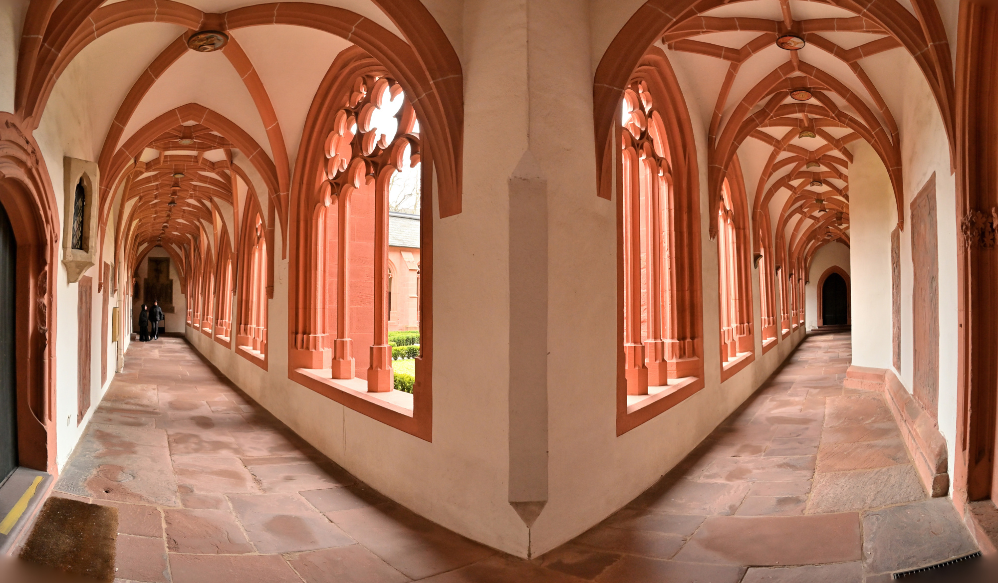
Kreuzgang-Eckpanorama

1/40s f/5,6 ISO 640/29° f=7,5mm
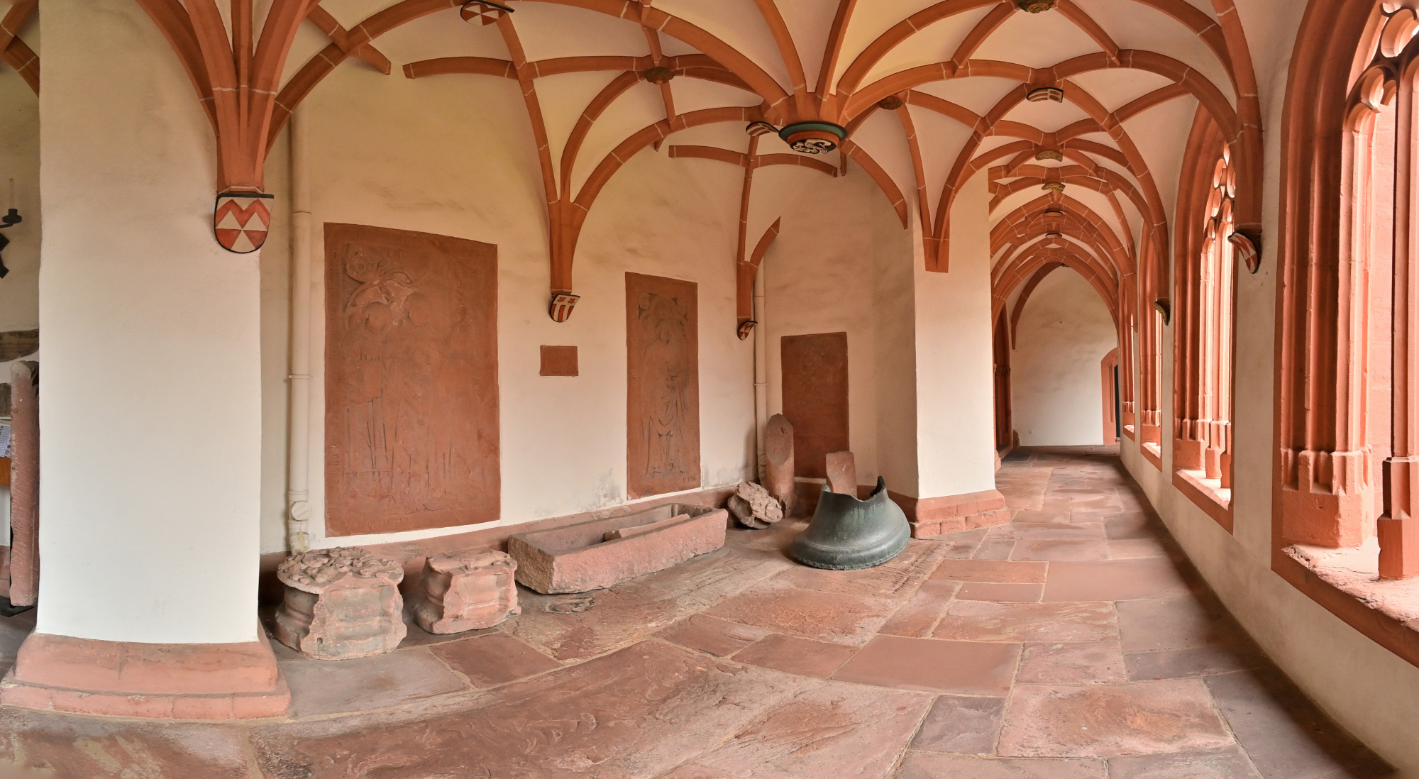
1/40s f/5,6 ISO 100/21° f=7,5mm
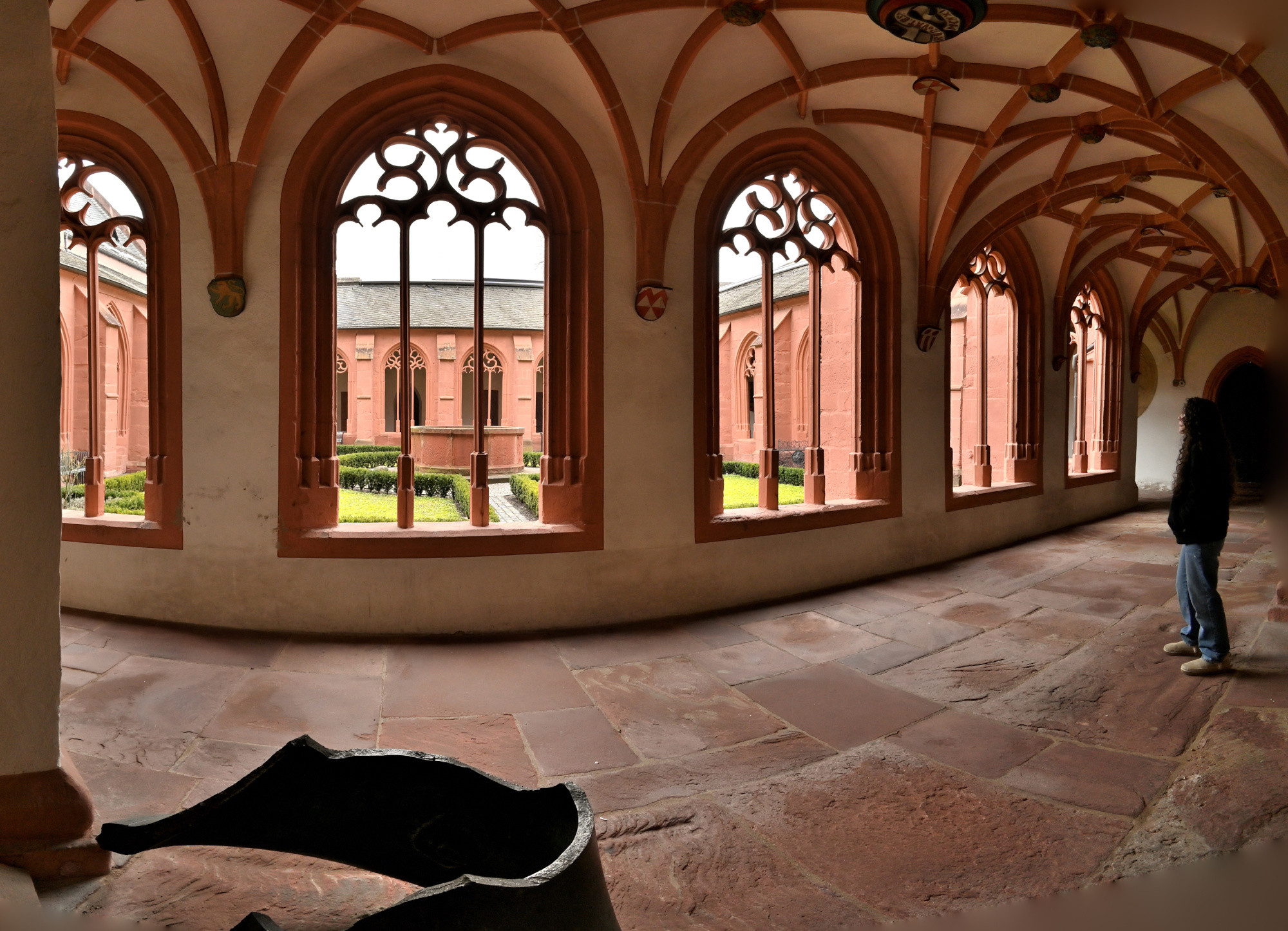
1/40s f/5,6 ISO 2000/34° f=7,5mm
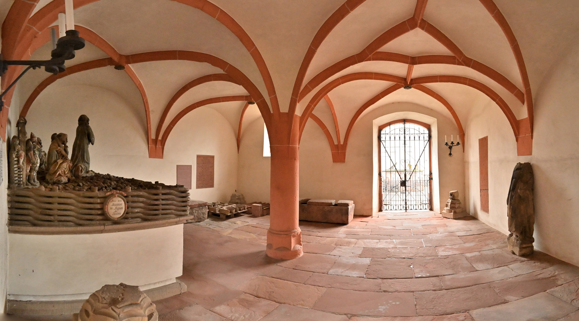
Interaktives Panorama Kreuzgang 1 360x180
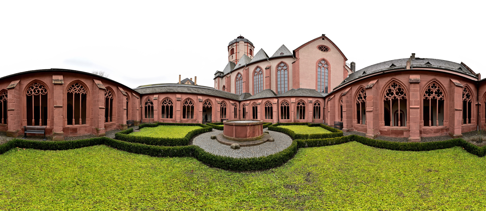
1/50s f/2 ISO 100/21° f=7,5mm

Interaktives Panorama Kreuzgang 2 360x180
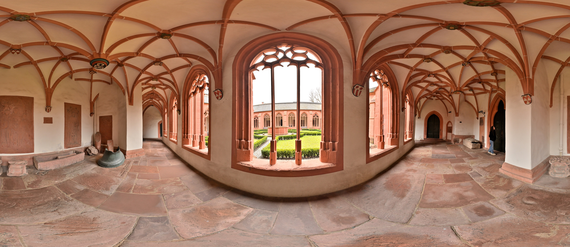
1/50s f/2 ISO 100/21° f=7,5mm

Außenansicht
1/160s f/5,6 ISO 100/21° f=7,5mm
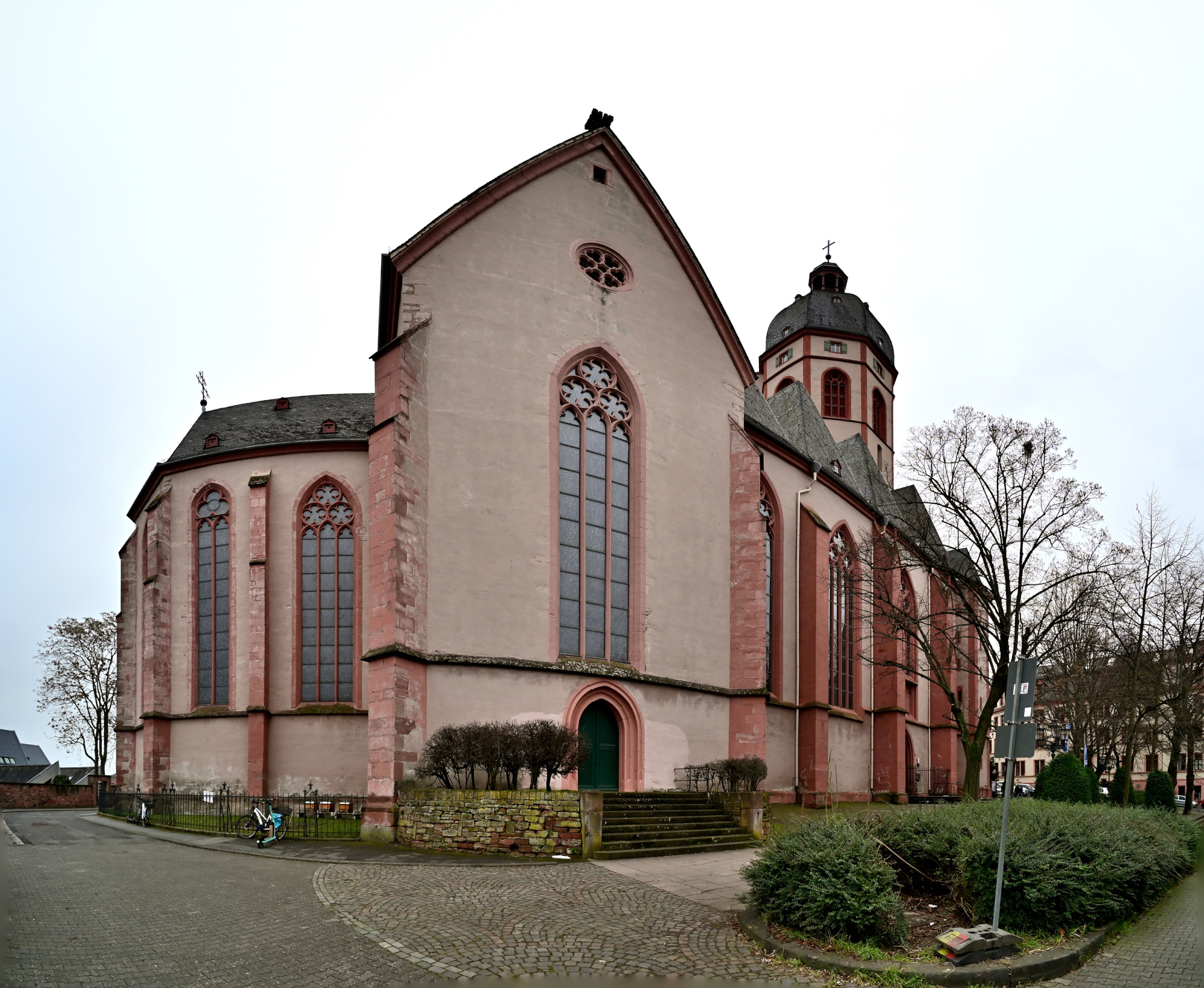
1/100s f/5,6 ISO 100/21° f=7,5mm
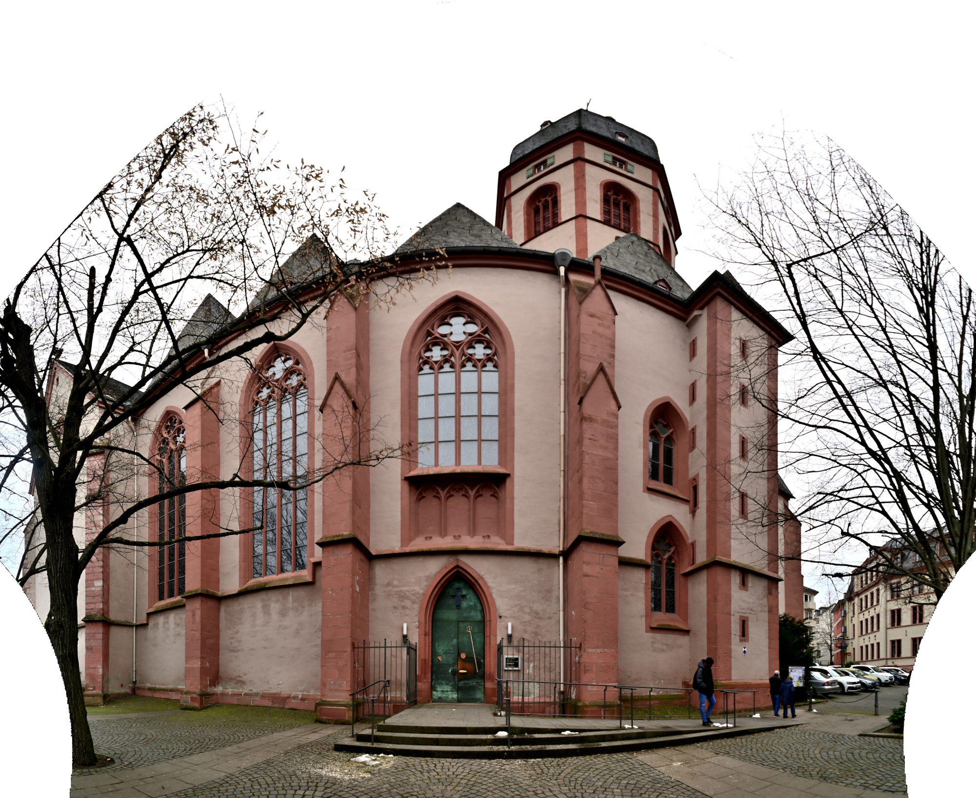
Mercator-Projektionen von: